Week 9 - Parametric study on Gate valve.

PARAMETRIC STUDY ON GATE VALVE

Aim: Simulate the Gate valve using Parametric study.

Objectives:

• Obtain the mass flow rates at the outlet for each design point.
• Calculate the flow coefficient and flow factor for each opening and plot the graph.
• Discuss the results of the mass flow rate and flow coefficient.

Introduction:

A gate valve is the most common valve for water supply systems. It represents a linear-motion isolation valve and has a function to stop or allow the flow. Gate valves got their name from the closure element sliding into the flow stream to provide shutoff and, therefore, acting like a gate. Gate valves are used to isolate specific areas of the water supply network during maintenance, repair works, new installations, as well as to reroute water flow throughout the pipeline.

A gate valve has a simple design and can be applied in many low pressure-drop services, which makes it one of the most common valves in use today. Gate valves are designed as full-port valves. This means that the valve port is of the same size as the inner diameter of the connecting pipe. Full-bore gate valve passes the fluid flow without any obstructions to a flow and do not cause a pressure drop in a pipeline. This also allows to clean the pipe using a cleaning pig.

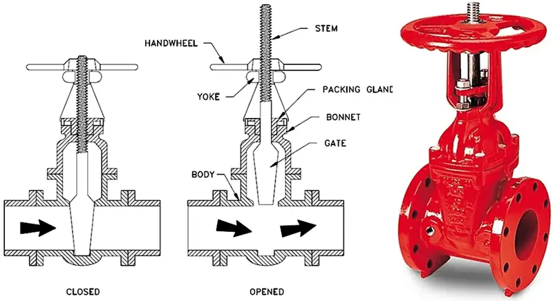
Gate valves are normally operated by a handwheel, a valve T-key (wrench) or an actuator. The wheel is attached to a valve stem and transfers rotational energy to it. During the gate valve opening, the rotation of the handwheel turns the threads of the gate stem into the gate and vice versa for closing. This energy moves the gate valve wedge downwards or upwards. In underground gate valve installations, an extension spindle is attached, which allows operation without direct access to the valve itself.

Applications of Gate-valve:

• Socket or butt-welding end-gate valves in air, fuel gas, feedwater, steam, lube oil, and other systems are typical applications.
• Threaded-end gate valves may be used in air, gaseous, or liquid systems.
• Concern for leakage from threaded connection can be addressed by seal welding the threaded connection or by using thread sealants, as appropriate. In low-pressure and low-temperature systems such as fire protection systems’ water piping or water distribution pipelines, flanged gate valves are commonly used.

Procedure/steps involved to perform the simulation:

1. Geometry creation:

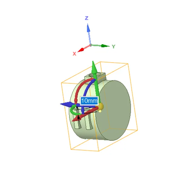
We need the load/Import the geometry to spaceclaim, then need to extract the fluid volume from 3D gate valve. Then we have to lift the gate disc with 10mm with the help of move option which is available in design taskbar.

Create the parameter in group section which will be set as 10mm lift.

Create 2d /Section view to Gate Valve, There will some gap between fluid volume to lift of disc, to collapse them we use the 'update volume body in context' option to fit with each other.

Enable Suppress for physics to all the solid components. Select the pull option available in design taskbar and select at side of valve to extend the valve with pipe of 800mm on both sides.

After extend of pipe pressing on volume we get the 'upadte volume body in context' click to fit the volume to extended pipe.

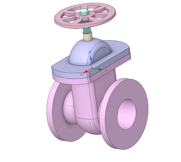
3D Geometry of Gate valve:

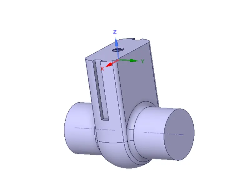
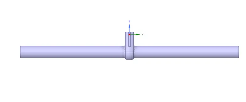
Volume extracted body of Gate valve:

Lift of Gate disc of 10mm:

Sectioned view of Gate valve with 10mm lift:

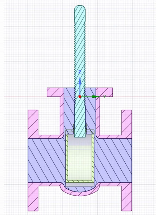
Assembly of Gate valve and Pipe:

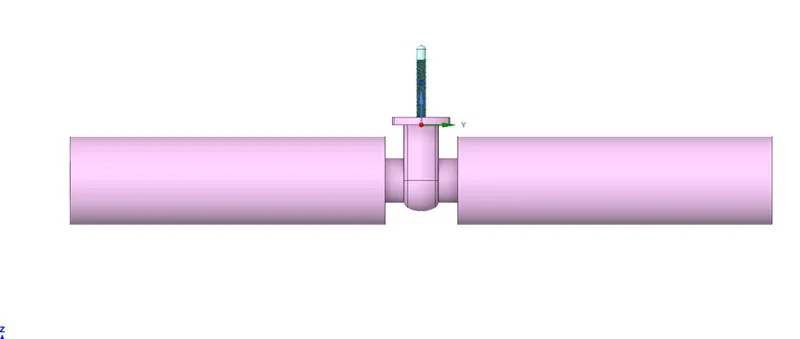
Assembly of Gate valve and Pipe (Fluid volume):

Mesh:

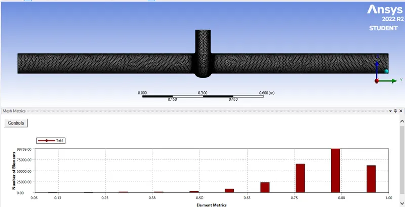
Importing the fluid volume of gate valve body into meshing section. We applied the Mesh size as 0.008m (8mm) size. With that mesh size we get elements of 258081 and nodes of 53196. Name the inlet and outlet to pipe.

Meshed body:

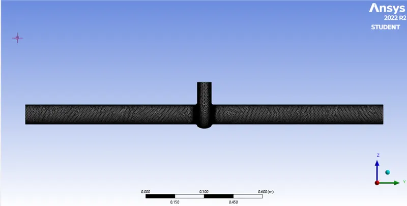
Mesh with element quality:

Setup:

In this section we have to set the conditions and parameters to simulate the Gate valve simulation. We use the pressure-based solver with steady state time management and we use the gravitational acceleration in negative z-direction as -9.81.

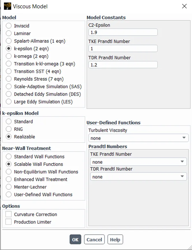
For this particular Gate valve simulation, we use k-epsilon with realizable model with scalable wall functions of viscous model. Coz in this case the Reynolds number is above 2000 and is in turbulent flow.

For Reynolds number we have

Re = ρ*u*D/μ

ρ = Fluid density

μ = Dynamic viscosity

u = Velocity of flow

D Diameter of pipe

Re = 998.8 * 0.1415488 * 0.1/0.001

Re = 14137.89

Since the above Re value is greater than 2000.

From above Reynolds we considered the viscous model.

We selected material as water which flow into Gate valve pipe and we removed the air material to avoid the mixture of water and air material.

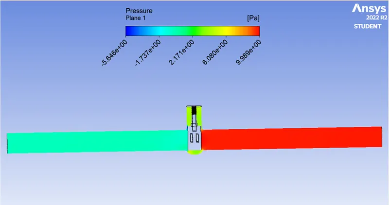
The boundary conditions are at inlet and outlet we considered as pressure-inlet and pressure-outlet type flow into pipe. At pressure-inlet apply 10Pa as Gauge factor pressure and at pressure-outlet keep it as 0Pa pressure Gauge factor.

Allowing the solution method as coupled method with second order-upwind at turbulent kinetics and turbulent dissipation rate.

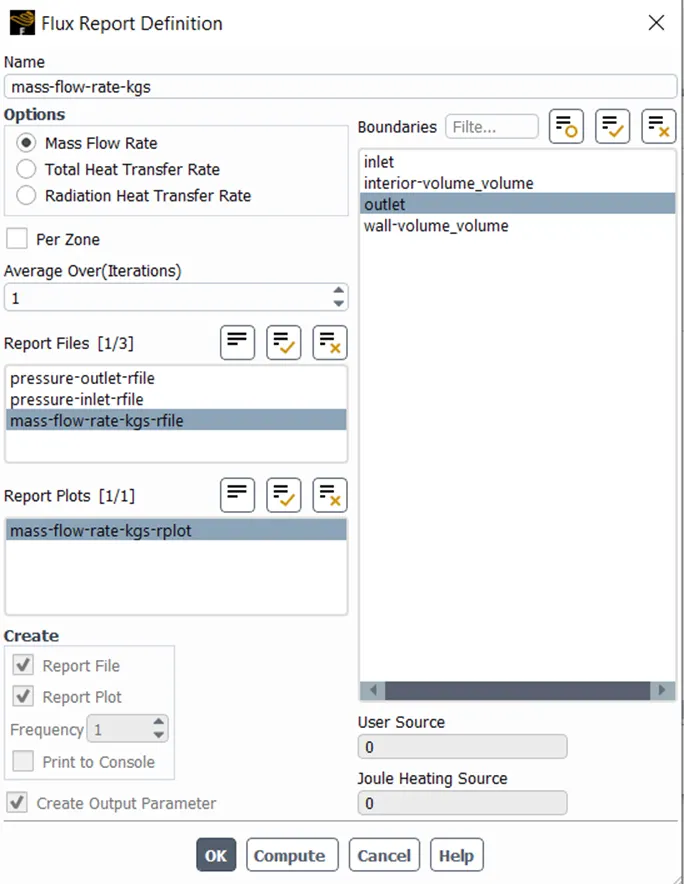
Create the mass-flow-rate at outlet of the pipe body.

Initializing with standard condition which will compute from inlet, create contour on YZ plane which will created on body.

Run the simulation for 10mm lift of disc.

Simulation at lift of 10mm:

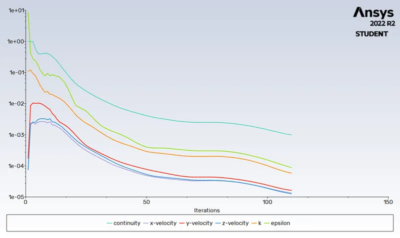
Residual Plot:

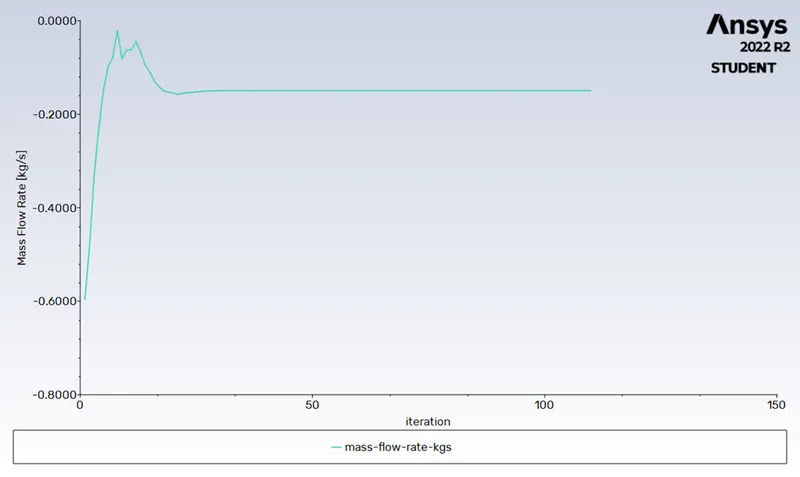
Mass flow rate:

Flow coefficient:

The flow coefficient of a device is a relative measure of its efficiency at allowing fluid flow. It describes the relationship between the pressure drop across an orifice valve or other assembly and the corresponding flow rate.

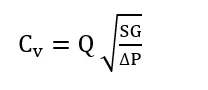
Mathematically the flow coefficient Cv can be expressed as:

Where,

Q - Rate of flow (expressed in US gallons per minute),

SG - Specific gravity of the fluid (for water = 1),

ΔP - Pressure drop across the valve (expressed in psi).

Flow Factor (Kv) :

The flow of water with temperature ranging 5-30*C through a valve in cubic meters per hour m^3/h with a pressure drop of 1 bar.

The relationship between flow coefficient and flow factor can be expressed as:

Kv = 0.865.Cv

We calculated the flow coefficient and flow Factor for 10 mm lift

mass flow rate = 0.14953 kg/sec, 1kg/sec=15.85 gal/min , Q = 2.370 gal/min

SG (specific gravity) for water = 1

ΔP = Pressure at inlet - pressure at outlet = 9.817Pa, 1pa =0.000145psi

ΔP =0.00142 psi

Put these values in eq (1)

Cv = 62.893

put this value in eq (2) we get

Kv = 54.402

Post-Process:

Pressure acting on plane:

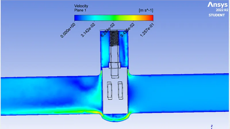
Velocity of flow in pipe:

Simulation at lift of 20mm:

Residual plot:

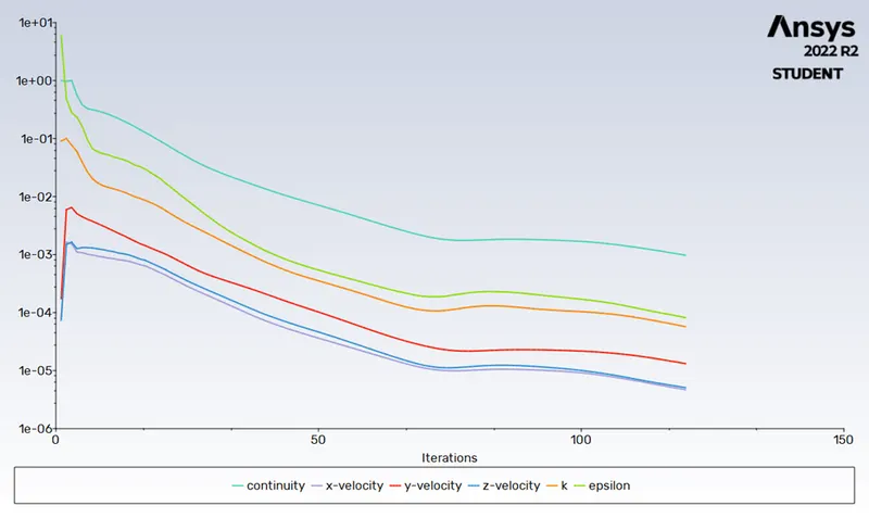
Mass flow rate:

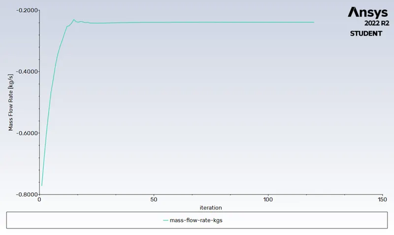
We calculated the flow coefficient and flow Factor for 20 mm lift

mass flow rate = 0.2394 kg/sec, 1kg/sec=15.85 gal/min, Q = 3.79449 gal/min

SG (specific gravity) for water = 1

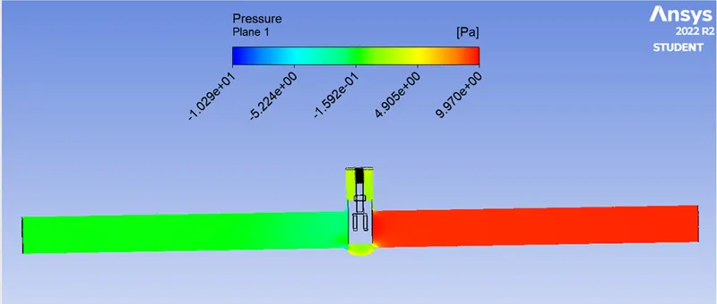
ΔP = Pressure at inlet - pressure at outlet = 9.531Pa, 1pa =0.000145psi

ΔP =0.00138 psi

Put these values in eq (1)

Cv = 102.144

put this value in eq (2) we get

Kv = 88.354

Pressure acting on plane:

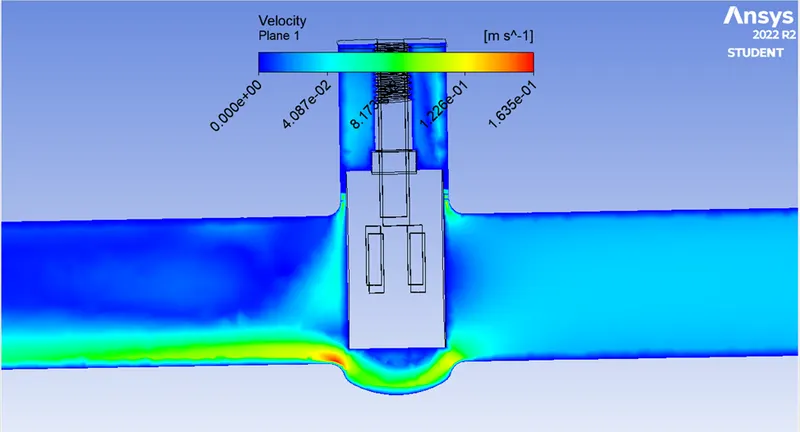
Velocity of flow in pipe:

Simulation at lift of 30mm:

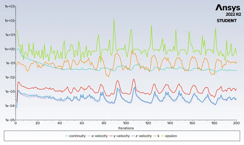
We calculated the flow coefficient and flow Factor for 30 mm lift

mass flow rate = 0.36019 kg/sec, 1kg/sec=15.85 gal/min , Q = 5.709 gal/min

SG (specific gravity) for water = 1

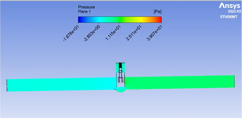
ΔP = Pressure at inlet - pressure at outlet = 8.932 Pa, 1pa =0.000145psi

ΔP =0.0013398 psi

Put these values in eq (1)

Cv = 155.96

put this value in eq (2) we get

Kv = 134.91

Pressure acting on plane:

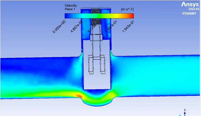
Velocity of flow in pipe:

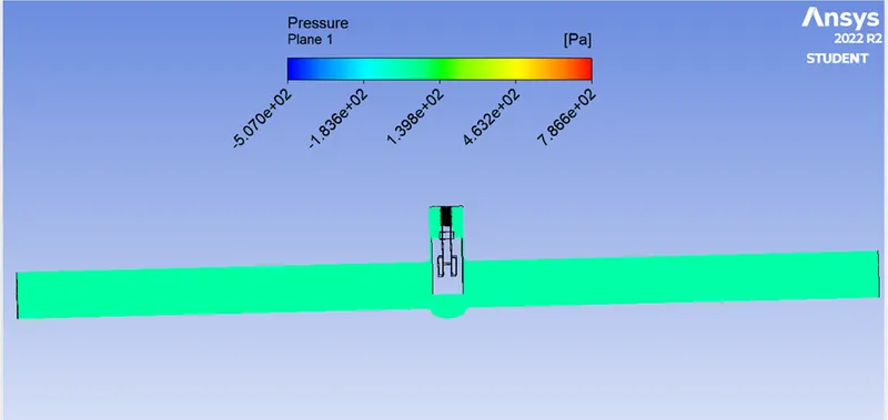
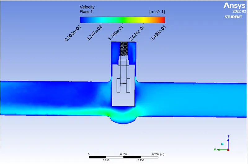
Simulation at lift of 40mm:

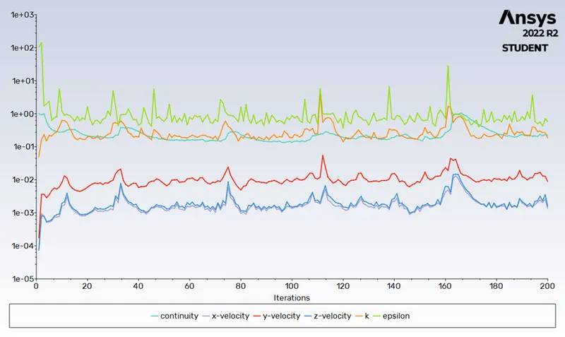
Residual plot:

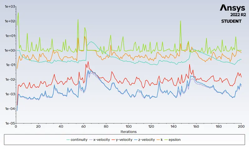
We calculated the flow coefficient and flow Factor for 40 mm lift

mass flow rate = 0.46618 kg/sec, 1kg/sec=15.85 gal/min , Q = 7.388 gal/min

SG (specific gravity) for water = 1

ΔP = Pressure at inlet - pressure at outlet =8.225Pa, 1pa =0.000145psi

ΔP =0.00119 psi

Put these values in eq (1)

Cv = 214.16

put this value in eq (2) we get

Kv = 185.25

Pressure acting on plane:

Velocity of flow in pipe:

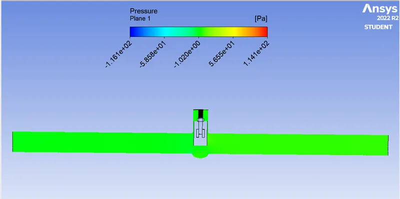
Simulation at lift of 50mm:

We calculated the flow coefficient and flow Factor for 50 mm lift

mass flow rate = 0.58206 kg/sec, 1kg/sec=15.85 gal/min , Q = 9.225651 gal/min

SG (specific gravity) for water = 1

ΔP = Pressure at inlet - pressure at outlet = 7.254Pa, 1pa =0.000145psi

ΔP =0.00105 psi

Put these values in eq (1)

Cv = 284.71

put this value in eq (2) we get

Kv = 246.28

Pressure acting on plane:

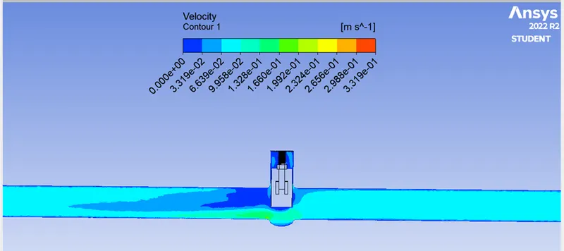
Velocity of flow in pipe:

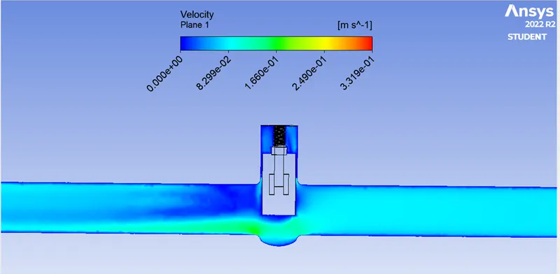
Contour plane in pipe:

Simulation at lift of 60mm:

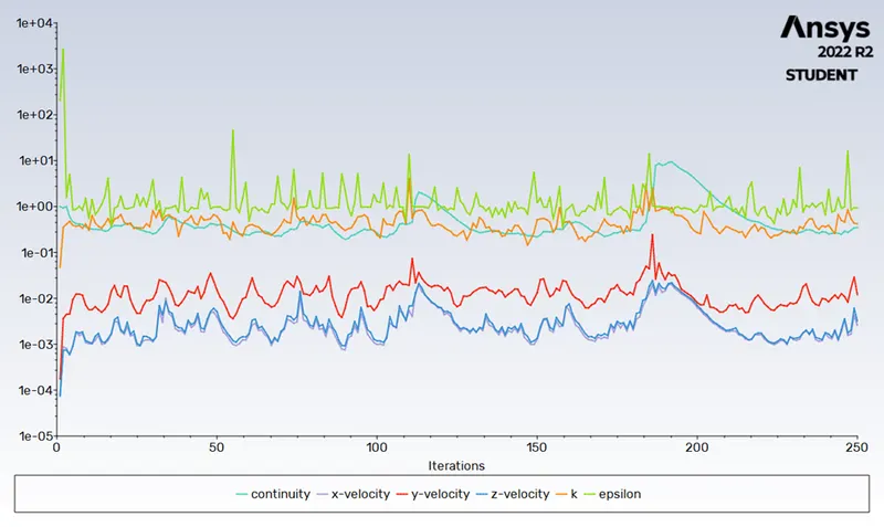
Residual plot:

We calculated the flow coefficient and flow Factor for 60 mm lift

mass flow rate = 0.70421 kg/sec, 1kg/sec=15.85 gal/min , Q = 11.1617285 gal/min

SG (specific gravity) for water = 1

ΔP = Pressure at inlet - pressure at outlet = 5.853 Pa, 1pa =0.000145psi

ΔP =0.000848 psi

Put these values in eq (1)

Cv = 383.29

put this value in eq (2) we get

Kv = 331.55

Pressure acting on plane:

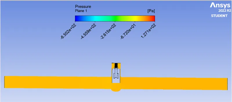
Velocity of flow in pipe:

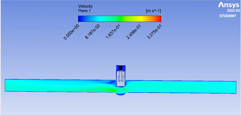
Vector with velocity on plane:

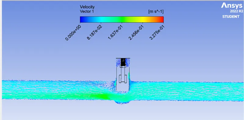
Simulation at lift of 70mm:

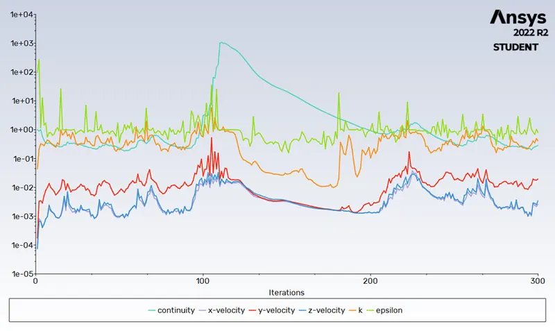
Residual plot:

We calculated the flow coefficient and flow Factor for 70 mm lift

mass flow rate = 0.72081 kg/sec, 1kg/sec=15.85 gal/min , Q = 11.424 gal/min

SG (specific gravity) for water = 1

ΔP = Pressure at inlet - pressure at outlet = 5.551Pa, 1pa =0.000145psi

ΔP =0.000804 psi

Put these values in eq (1)

Cv = 402.89

put this value in eq (2) we get

Kv = 348.50

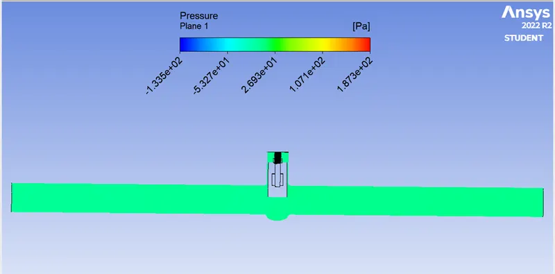
Pressure acting on plane:

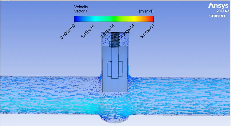
Velocity of flow in pipe:

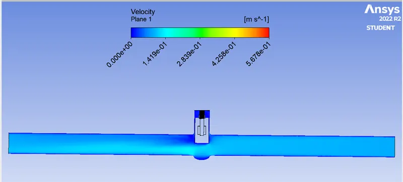
Vector plot with velocity in pipe:

Simulation at lift of 80mm:

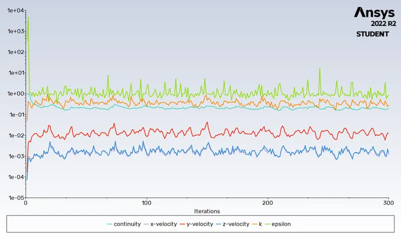
Residual plot:

We calculated the flow coefficient and flow Factor for 80 mm lift

mass flow rate = 0.8014 kg/sec, 1kg/sec=15.85 gal/min , Q = 12.702 gal/min

SG (specific gravity) for water = 1

ΔP = Pressure at inlet - pressure at outlet = 4.698 Pa, 1pa =0.000145psi

ΔP =0.000681 psi

Put these values in eq (1)

Cv = 486.74

put this value in eq (2) we get

Kv = 421.03

Pressure acting on plane:

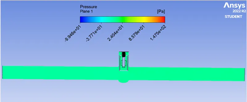
Velocity of flow in pipe:

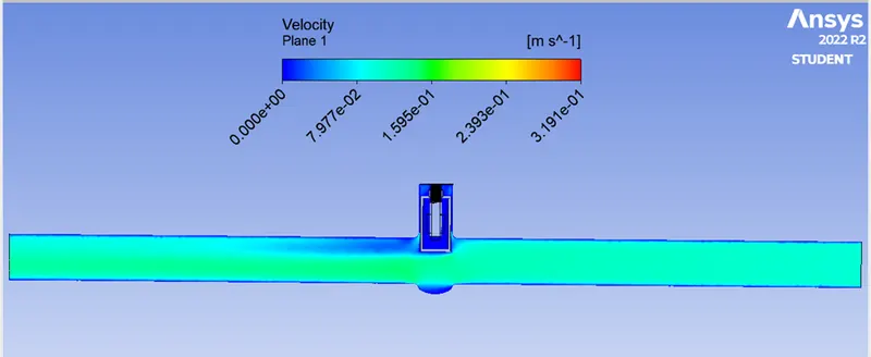
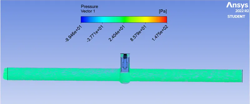
Vector plot with pressure:

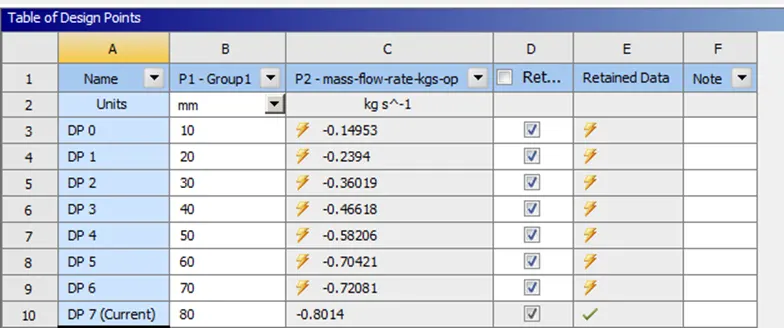
Parametric Result Table:

Observations:

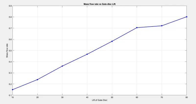
From the observation of result table, we can say that the mass flow rate is increases when we increase the gate disc lift of gate valve.

The mesh elements decrease as lift of gate disc of gate valve.

The pressure drop is also decreases when we increase the gate disc lift of gate valve.

The negative sign of the mass flow rate value is due to the mass flow which is leaving at the outlet.

The flow coefficient is also increases when we increase the gate disc lift of gate valve.

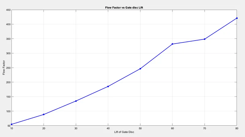
The flow factor is also increases when we increase the gate disc lift of gate valve.

Grid Dependence test on Gate valve simulation:

Design Points	Gate Disc Lift in mm	Mass-Flow-Rate in (Kg/s)	Flow co-efficient	Flow Factor
1	10	-0.14953	62.89	54.40
2	20	-0.2394	102.14	88.35
3	30	-0.36019	155.96	134.91
4	40	-0.46618	214.16	185.25
5	50	-0.58206	284.71	246.28
6	60	-0.70421	383.29	331.55
7	70	-0.72081	402.89	348.50
8	80	-0.8014	486.74	421.03

The Graphs plotted from MATLAB code

% Lift of disc 
Lift = [10 20 30 40 50 60 70 80];
% flow factor
Flow_Factor = [54.40 88.35 134.91 185.25 246.28 331.55 348.50 421.03];
% flow coefficient
Flow_Coefficient = [62.89 102.14 155.96 214.16 284.71 383.29 402.89 486.74];
% Mass flow Rate
Mass_Flow_Rate = [0.14953 0.2394 0.36019 0.46618 0.58206 0.70421 0.72081 0.8014];


% Plot
figure(1)
a1 = plot(Lift,Flow_Factor,'color','b','Marker','*','LineWidth',2); 
xlabel("Lift of Gate Disc")
ylabel("Flow Factor")
grid on
title("Flow Factor vs Gate disc Lift")

figure(2)
a2 = plot(Lift,Flow_Coefficient,'color','b','Marker','*','LineWidth',2);
xlabel("Lift of Gate Disc")
ylabel("Flow Coefficient")
grid on
title("Flow Coefficient vs Gate disc Lift")


figure(3)
a3 = plot(Lift,Mass_Flow_Rate,'color','b','Marker','*','LineWidth',2); 
xlabel("Lift of Gate Disc")
ylabel("Mass flow rate")
grid on
title("Mass flow rate vs Gate disc Lift")

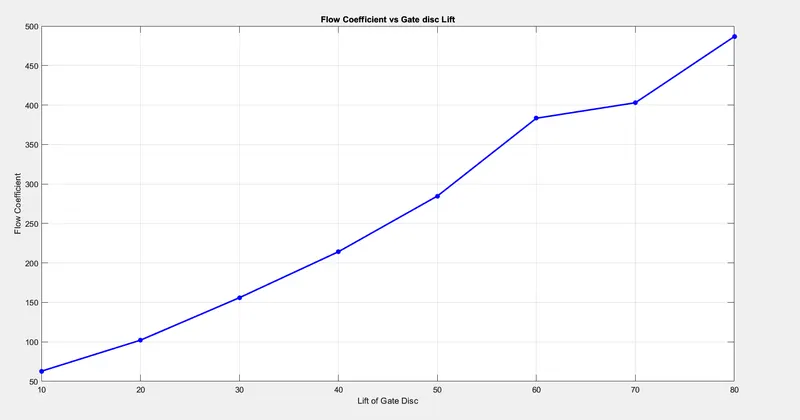
Gate valve lift vs Flow coefficient graph:

Gate valve lift vs Flow Factor graph:

Gate valve lift vs Mass Flow Rate graph:

Conclusion:

From above results and observations we conclude that, as the mass flow rate is increases if we increase the gate valve opening (gate disc lift) .

The velocity of the flow is also increases when we increase the gate disc lift of gate valve.

The pressure drop is decreases when we increase the gate disc lift of gate valve.

The graph of flow factor and flow coefficient with respect to lift of the gate valve is plotted.

The gate valve opening is increases then flow coefficient and flow factor is also increases.