Week 9 - Parametric study on Gate valve.
CHALLENGE REPORT :
AIM :
To perform a parametric study on the gate valve simulation by setting the opening from 10 % to 80%.
OBJECTIVE :
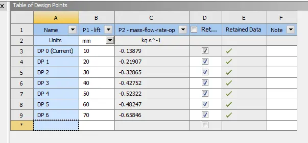
* To obtain the mass flow rates at the outlet for each design point.
* To calculate the flow coefficient and flow factor for each opening.
* Plot the graph and create contours for pressure and velocity.
* Discuss the results of the mass flow rate and flow coefficient.
INTRODUCTION :
GATE VALVE :
A gate valve, also known as a sluice valve, is a valve that opens by lifting a barrier (gate) out of the path of the fluid. Gate valves require very little space along the pipe axis and hardly restrict the flow of fluid when the gate is fully opened. The gate faces can be parallel but are most commonly wedge-shaped (in order to be able to apply pressure on the sealing surface).
Use:
Gate valves are used to shut off the flow of liquids rather than for flow regulation. When fully open, the typical gate valve has no obstruction in the flow path, resulting in very low flow resistance. The size of the open flow path generally varies in a nonlinear manner as the gate is moved. This means that the flow rate does not change evenly with stem travel. Depending on the construction, a partially open gate can vibrate from the fluid flow.
Gate valves are mostly used with larger pipe diameters (from 2" to the largest pipelines) since they are less complex to construct than other types of valves in large sizes.
At high pressures, friction can become a problem. As the gate is pushed against its guiding rail by the pressure of the medium, it becomes harder to operate the valve. Large gate valves are sometimes fitted with a bypass controlled by a smaller valve to be able to reduce the pressure before operating the gate valve itself.
Flow Co-efficient:
Kv can be calculated from Cv using the equation:
- `K_v = 0.865*C_v`
PROCEDURE :
GEOMENTRY SETUP :
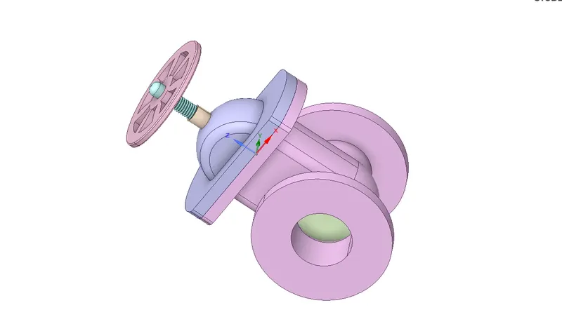
* Just import the model from the problem by opening the space claim .
* Extend the both pipes upto 800mm which is on the side of gate valve by using the pull option under the design.
Space claim ----> Design ----> pull ---->Pull towards z axis ----> Give the length as 800mm ----> ok
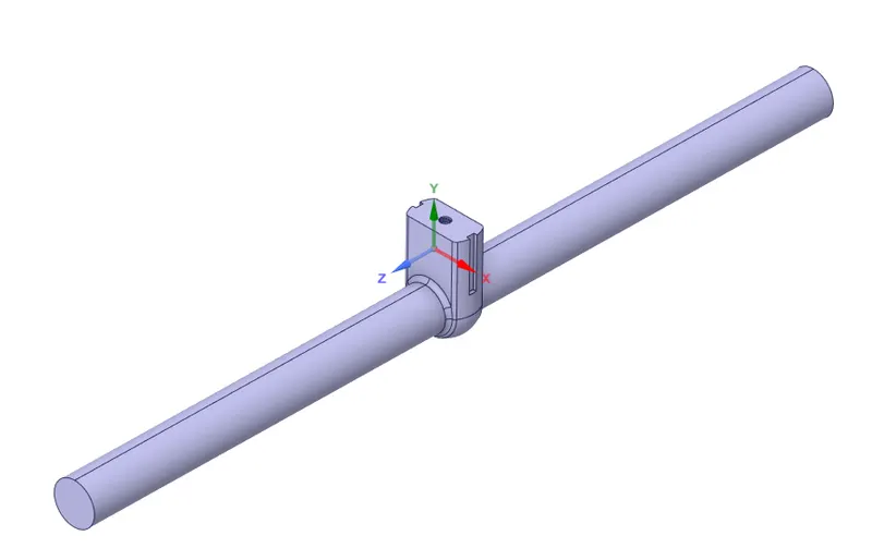
* Create the fluid volume by selecting the edges with the help of volume extract option under repair menu in the space claim.
* Using the Move option move the spindle and gate disc together and set as parameter in the group by using create parameter.
After moving ----> Group ----> Create parameter
* For all the components other than volume aplly the supress for physics, so that we can only have the extracted volume.
|
Imported 3D model |
|
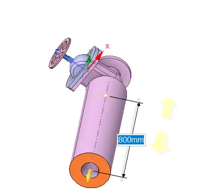
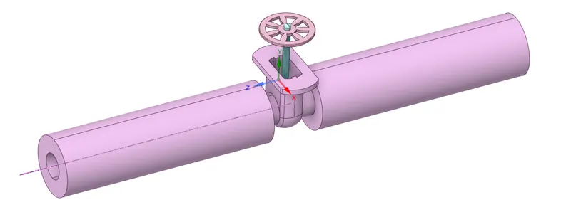
3D model inlet & exhaust has been extended
|
The fluid volume extracted using Volume extract option |
Extracted fluid volume |
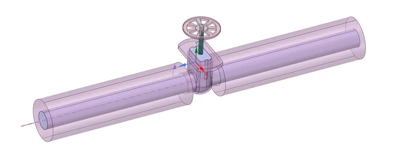
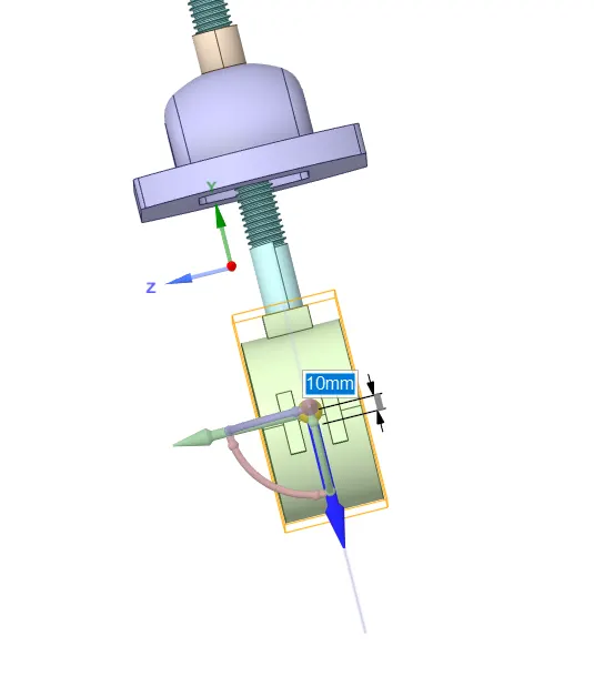
The opened valve of 10mm to calculate mass flow rate of water.
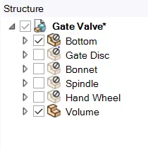
* As hight of valve opening is set as parameter, the simulation is carried out for 8 cases from 10mm to 80mm. The Parameter setup makes the simulation easier and time saving method.Case 1 = 10
- Case 2 = 20
- Case 3 = 30
- Case 4 = 40
- Case 5 = 50
- Case 6 = 60
- Case 7 = 70
- Case 8 = 80
MESH :
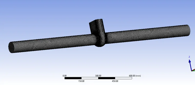
* Created geomentry is opened in the mesh module and give generate mesh.
* Given mesh size is 10mm and Update it.
Mesh (right click) ----> Mesh size as 10mm ----> Genarate mesh ----> update it
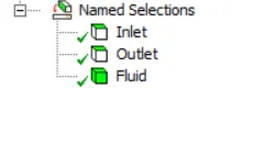
* Make the name selection by selecting the one face pipe as inlet and other faces as outlet and select total volume and name as fluid.
SETUP SOLUTION :
* After the mesh open the set up modul and here we have to set the condition like physics, boundery conditions, type of analysics, Solution setups and the requried outups.
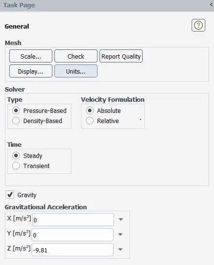
* Here enable the steady state solver because we don't need simulation results for each and every seconds so we need to consider the result of final stage. Pressure based is used because the velocity of air is low ( less than 0.3 of mach number ) and enable gravity with Z axis as -9.81 .
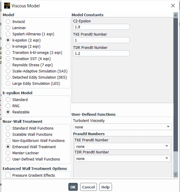
* Use K-epcelon model by opening the Viscous option in the physics and select the because it gives better results than RNS and Enhanced Wall Treatments under the near wall treatment is used.
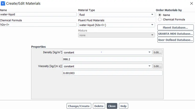
* Create the new material as water (H2O-liquid) from the fluid database in the material selection.
Physics ---> Materials ---> Fluid Data base ---> select the water ---> copy
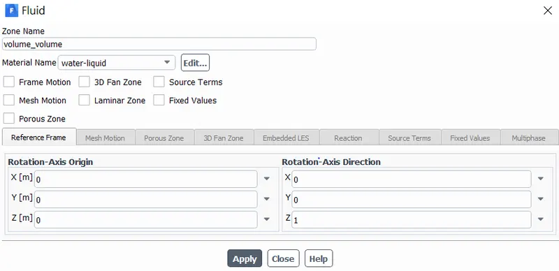
* In the cell zone set the water as the fluid for the fluid which is named in mesh.
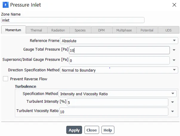
* Set the Boundries,
---> Inlet as Pressure inlet with 10 pa as Gauge total pressure.
---> Outlet as Pressure oullet with 0 pa as Gauge total pressure.
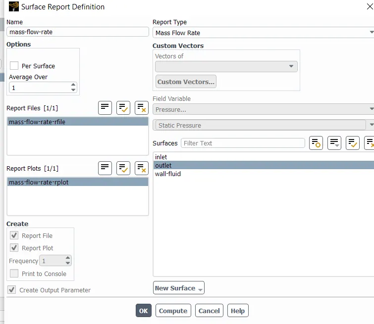
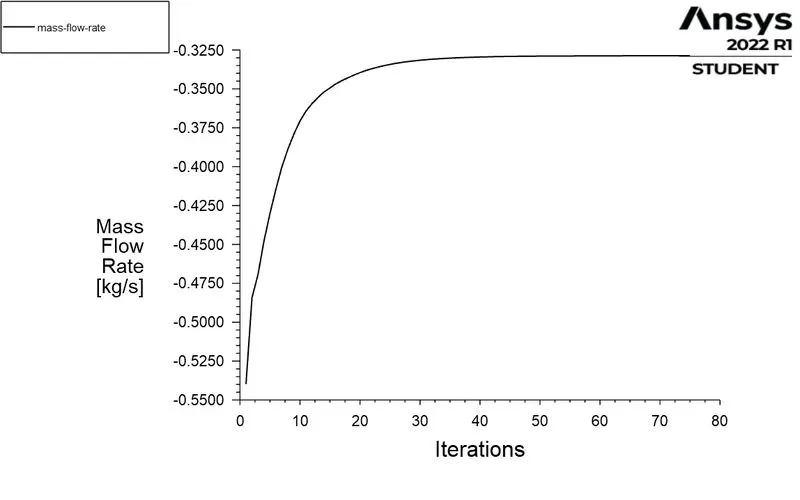
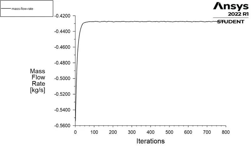
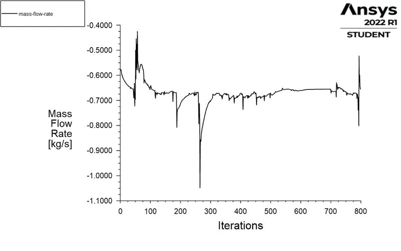
* Create the mass flow rate report from the definition under the solution tab.
Solution ---> Definition ---> new ---> Surface report ----> Mass flow rate ----> Outlet (ok)
* Initialize it with the Hybride initialization method.
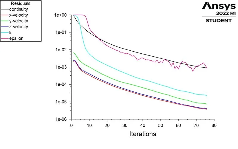
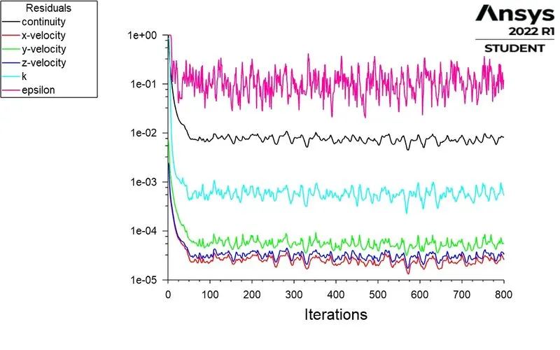
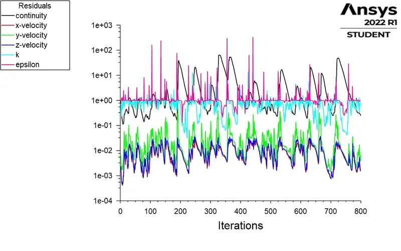
* Set the No of iteration as 1000 and start the calculation untill its converges.
MATERIAL CREATED :
CELL ZONE
BOUNDRIES :
CREATED REPORT :
CFD POST :
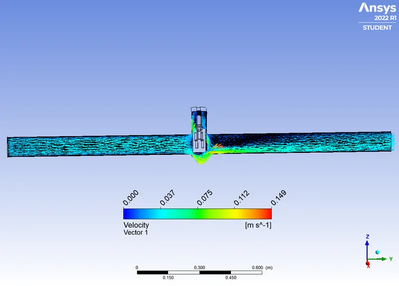
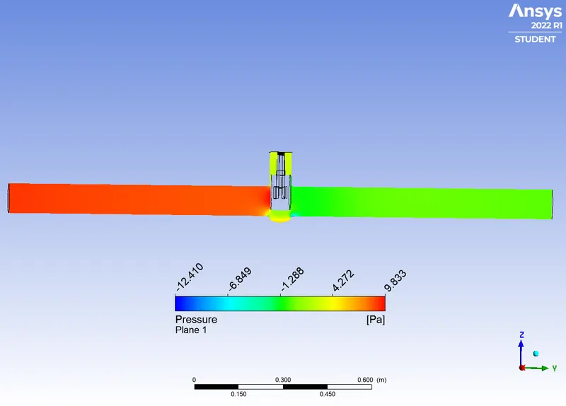
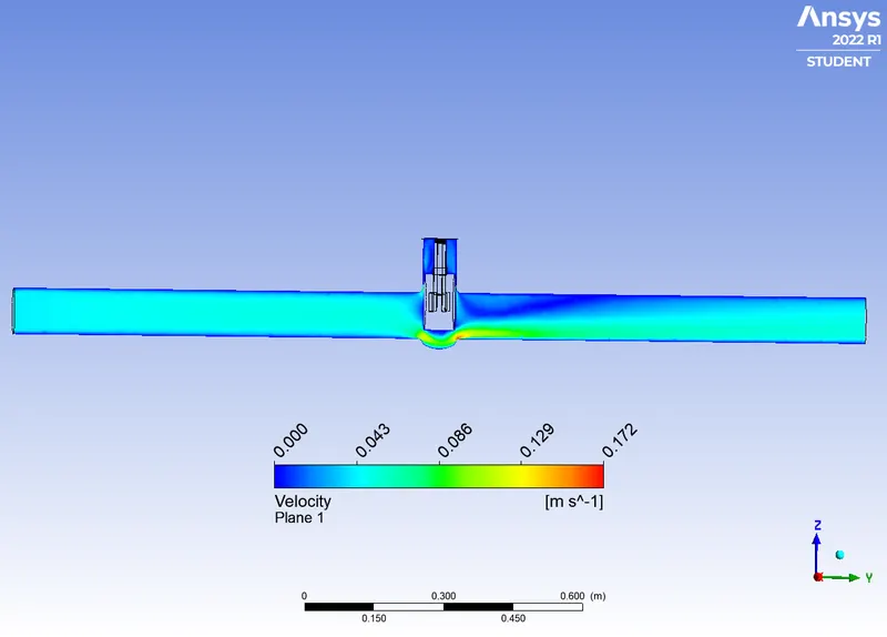
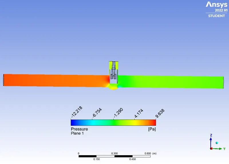
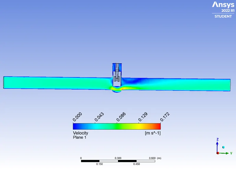
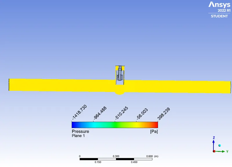
* Create the Pressure contours and velocity contours.
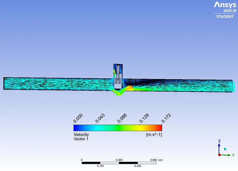
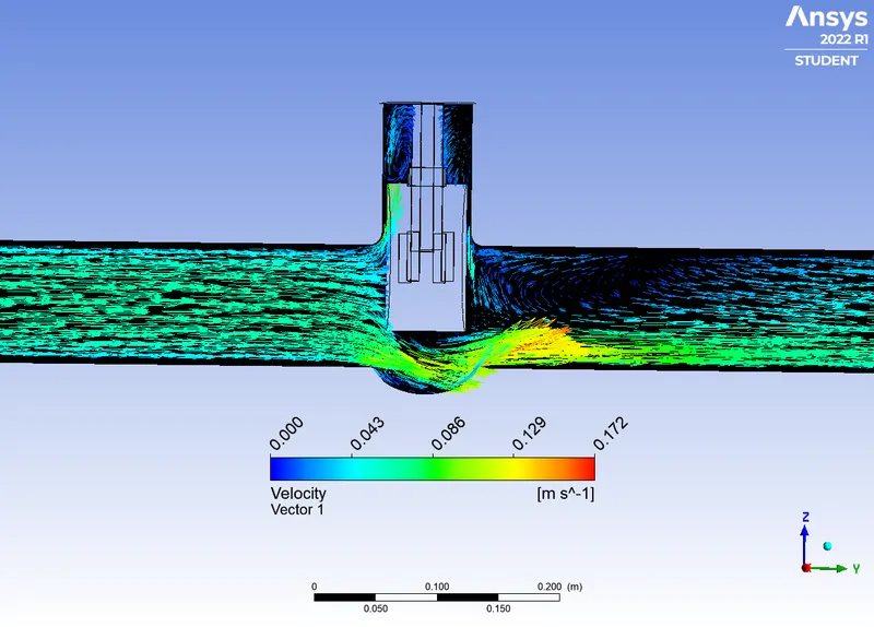
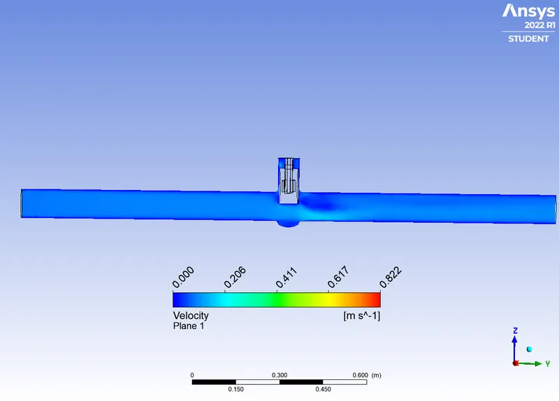
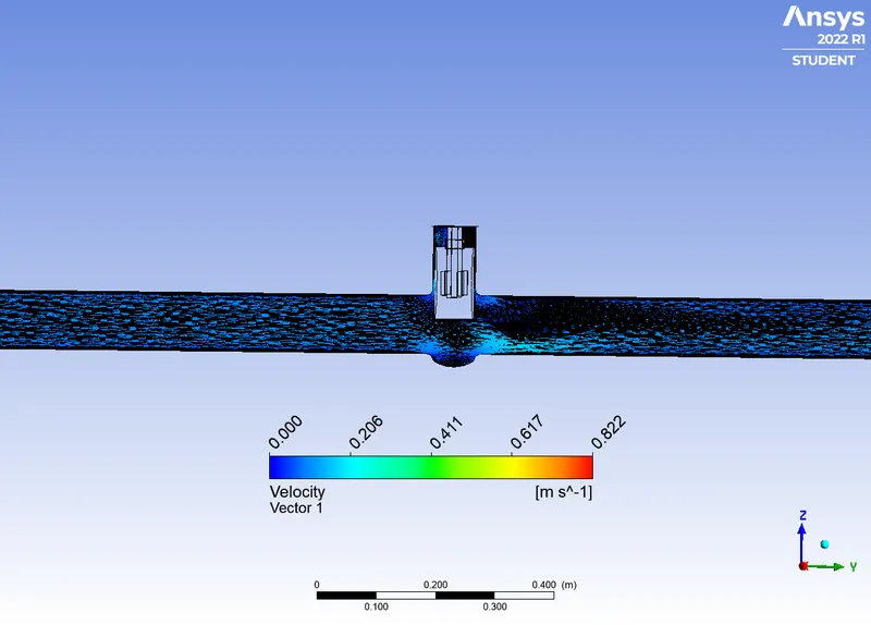
* Create the velocity vectors.
RESULTS :
CASE 1 :
lIFT = 10mm
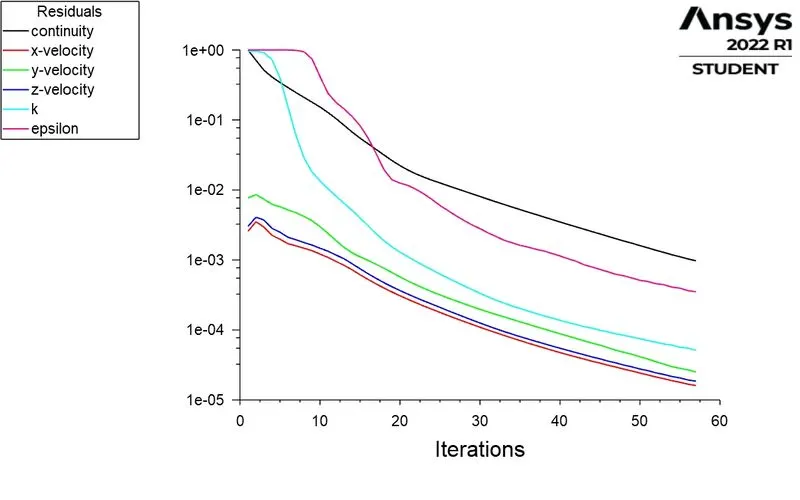
RESIDUAL PLOT :
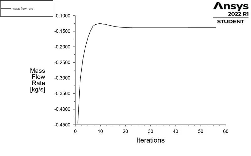
MASS FLOW RATE :
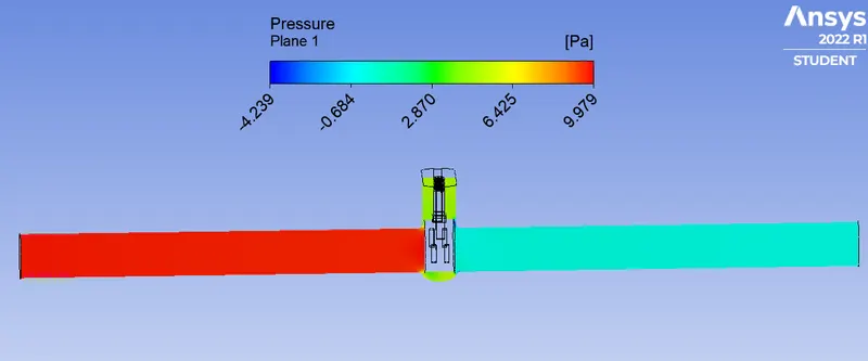
PRESSURE CONTOUR :
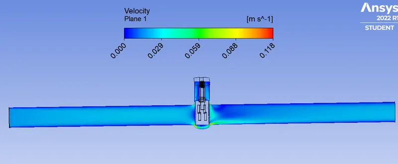
VELOCITY CONTOUR :
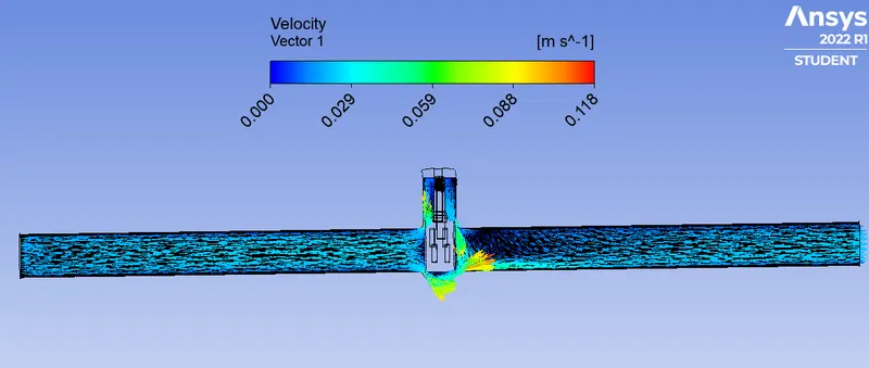
VELOCITY VECTOR :
CASE 2 :
lIFT = 20mm
RESIDUAL PLOT :
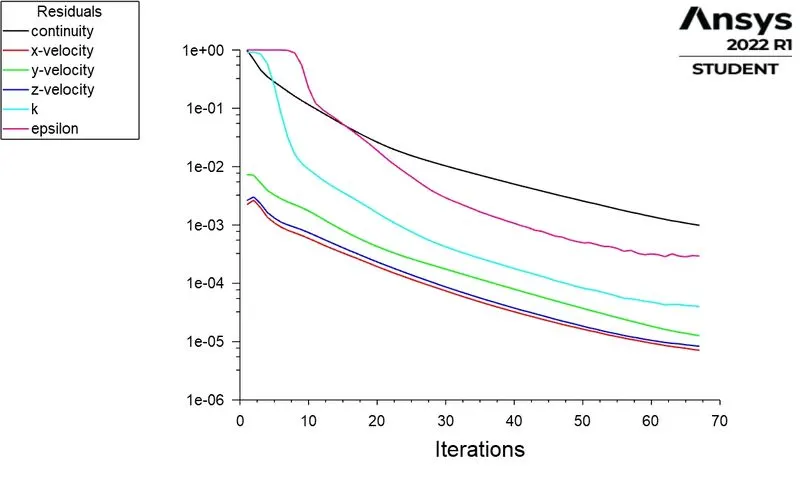
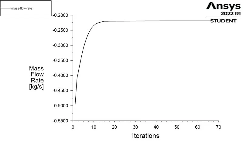
MASS FLOW RATE :
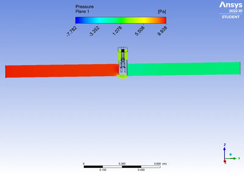
PRESSURE CONTOUR :
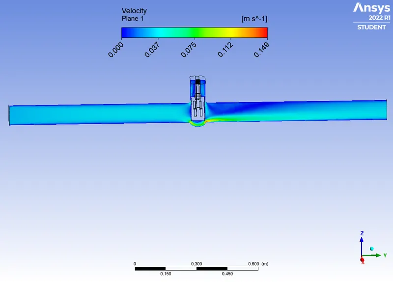
VELOCITY CONTOUR :
VELOCITY VECTOR :
CASE 3 :
lIFT = 30mm
RESIDUAL PLOT :
MASS FLOW RATE :
PRESSURE CONTOUR :
VELOCITY CONTOUR :
VELOCITY VECTOR :
CASE 4 :
lIFT = 40mm
RESIDUAL PLOT :
MASS FLOW RATE :
PRESSURE CONTOUR :
VELOCITY CONTOUR :
VELOCITY VECTOR :
CASE 5 :
lIFT = 50mm
RESIDUAL PLOT :
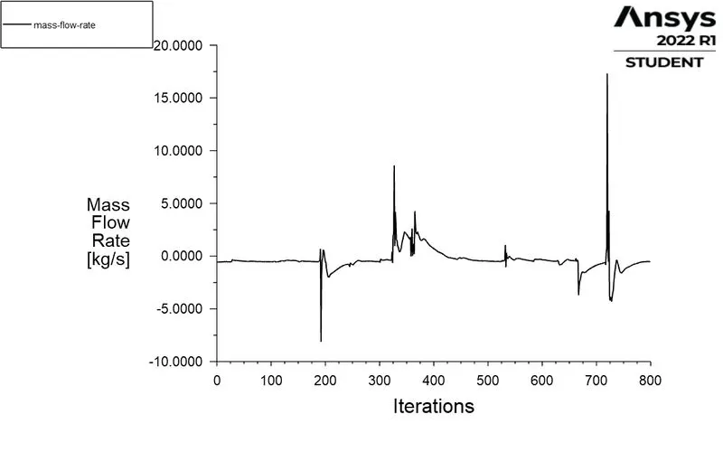
MASS FLOW RATE :
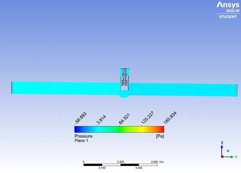
PRESSURE CONTOUR :
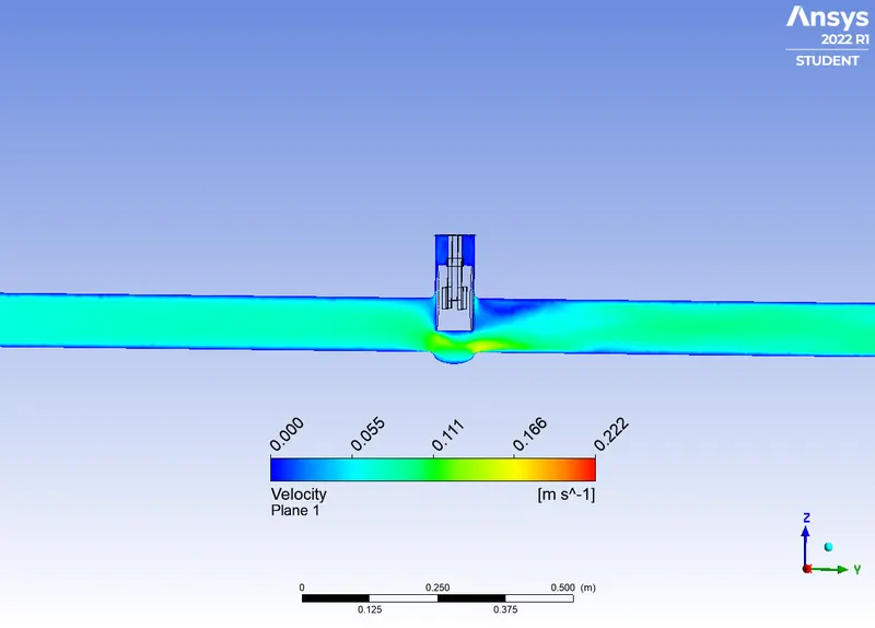
VELOCITY CONTOUR :
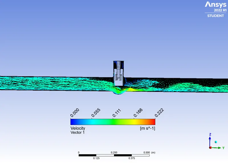
VELOCITY VECTOR :
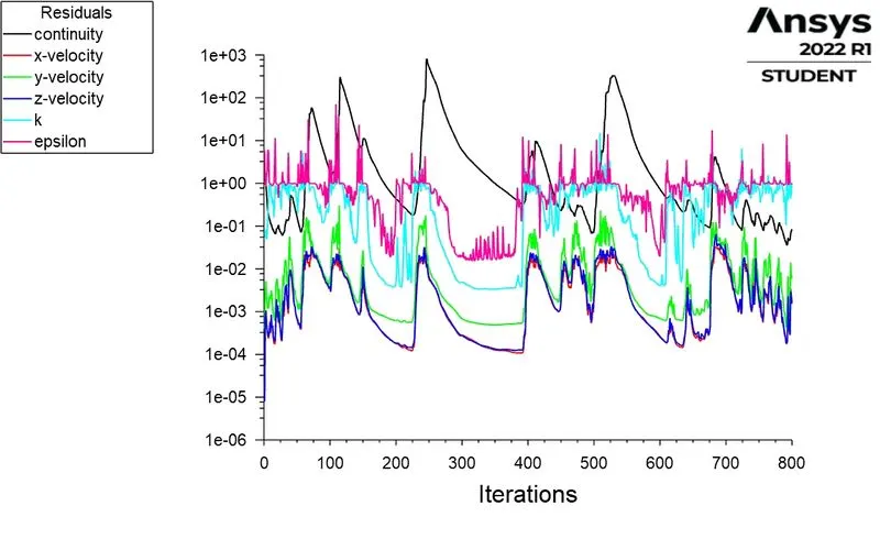
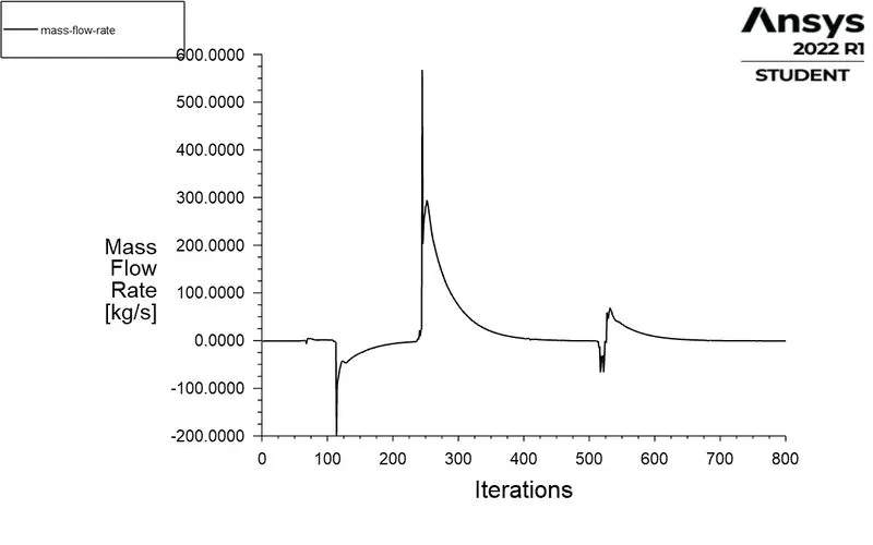
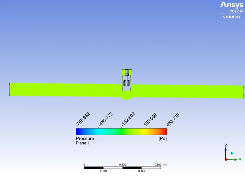
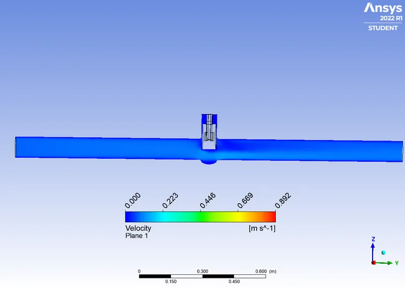
CASE 6 :
lIFT = 60mm
RESIDUAL PLOT :
MASS FLOW RATE :
PRESSURE CONTOUR :
VELOCITY CONTOUR :
VELOCITY VECTOR :
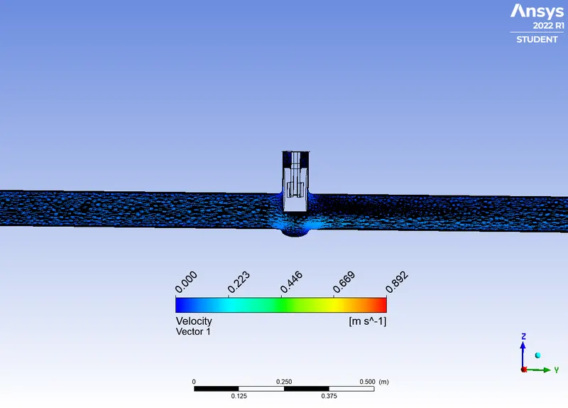
CASE 7 :
lIFT = 70mm
RESIDUAL PLOT :
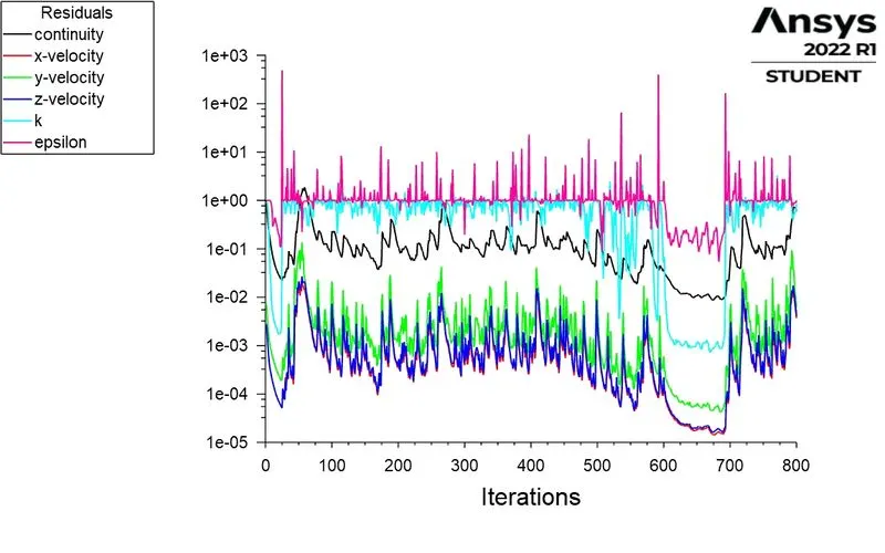
MASS FLOW RATE :
PRESSURE CONTOUR :
VELOCITY CONTOUR :
VELOCITY VECTOR :
CALCULATION FOR FLOW CO-EFFICIENT AND FLOW FACTOR :
Flow Co-efficient:
- `K_v = 0.865*C_v`
CASE 1 :
Mass flow rate =0.1387 kg/sec ( 1kg/sec=15.85 gal/min )
Q = 2.19839 gal/min.
SG (specific gravity) for water =1
ΔP = Pressure at inlet - pressure at outlet = 9.827pa , ( 1pa =0.000145psi )
ΔP =0.00142 psi.
Flow Co-efficient, C_V = 58.336
Flow Factor, K_V = 0.865 * 58.336
= 50.46064
CASE 2 :
Mass flow rate =0.21907 kg/sec ( 1kg/sec=15.85 gal/min )
Q =3.4722 gal/min.
SG (specific gravity) for water =1
ΔP = Pressure at inlet - pressure at outlet =9.5800 pa , ( 1pa =0.000145psi )
ΔP =0.00138 psi .
Flow Co-efficient, C_V = 93.46848
Flow Factor, K_V = 0.865 * 93.468
= 80.8501
CASE 3 :
Mass flow rate =0.32865 kg/sec ( 1kg/sec=15.85 gal/min )
Q =5.2091 gal/min.
SG (specific gravity) for water =1
ΔP = Pressure at inlet - pressure at outlet =9.112654 pa , ( 1pa =0.000145psi )
ΔP =0.001321 psi .
Flow Co-efficient, C_V = 143.3214
Flow Factor, K_V = 0.865 * 143.3214
= 123.973
CASE 4 :
Mass flow rate =0.42752 kg/sec ( 1kg/sec=15.85 gal/min )
Q =6.77619 gal/min.
SG (specific gravity) for water =1
ΔP = Pressure at inlet - pressure at outlet = 8.7734 pa , ( 1pa =0.000145psi )
ΔP =0.00127 psi .
Flow Co-efficient, C_V = 190.1439
Flow Factor, K_V = 0.865 * 190.1439
= 164.4745
CASE 5 :
Mass flow rate =0.52322 kg/sec ( 1kg/sec=15.85 gal/min )
Q =8.29303 gal/min.
SG (specific gravity) for water =1
ΔP = Pressure at inlet - pressure at outlet =7.795165 pa , ( 1pa =0.000145psi )
ΔP =0.0011302 psi .
Flow Co-efficient, C_V = 246.6809
Flow Factor, K_V = 0.865 * 246.6809
= 213.3789
CASE 6 :
Mass flow rate =0.604153 kg/sec ( 1kg/sec=15.85 gal/min )
Q =9.57582 gal/min.
SG (specific gravity) for water =1
ΔP = Pressure at inlet - pressure at outlet =6.86595 pa , ( 1pa =0.000145psi )
ΔP =0.00099562 psi .
Flow Co-efficient, C_V = 303.4793
Flow Factor, K_V = 0.865 * 303.4793
= 262.5095
CASE 7 :
Mass flow rate =0.65846 kg/sec ( 1kg/sec=15.85 gal/min )
Q =10.4365 gal/min.
SG (specific gravity) for water =1
ΔP = Pressure at inlet - pressure at outlet =6.379955 pa , ( 1pa =0.000145psi )
ΔP =0.000925092 psi .
Flow Co-efficient, C_V = 343.13331
Flow Factor, K_V = 0.865 * 343.13331
= 296.81031
TABLE FOR THE RESULT :
| CASES | LIFT | MASS FLOW RATE | FLOW COEFFICIENT | FLOW FACTOR |
| 1 | 10 mm | -0.13879 | 58.336 | 50.46064 |
| 2 | 20 mm | -0.21907 | 93.46848 | 80.8501 |
| 3 | 30 mm | -0.32865 | 143.3214 | 123.973 |
| 4 | 40 mm | -0.42752 | 190.1439 | 164.4745 |
| 5 | 50 mm | -0.52322 | 246.6809 | 213.3789 |
| 6 | 60 mm | -0.60415 | 303.4793 | 262.5095 |
| 7 | 70 mm | -0.65846 | 343.13331 | 296.81031 |
OBSERVATION :
* From the table we can observe that Mass flow rate increase with the increase of Disc lift of the Gate valve.
* The negavite sign of mass flow rate denotes that the fluid discharges through outlet of Gate valve.
* The pressure drop also decrease as the lift of disc increases.
* The flow coefficient is also increases when we increase the gate disc lift of gate valve.
* The flow factor is also increases when we increase the gate disc lift of gate valve.
* Higher mass flow rate is achieved at the 70mm disc lift.
CONCLUSION :
* The mass flow rate is increases with increase of gate valve opening (gate disc lift) .
* The velocity of the flow is also increases as we increase the disc lift of gate valve.
* The pressure drop is decreases with increase the gate disc lift of gate valve.
* The gate valve opening is increases then flow coefficient and flow factor is also increases.
* The design point 80 mm is not calculated because result obtained is not accurate and the reason behind that is the bug in ansys student version.