Week 9 - Parametric study on Gate valve.
Aim – To perform a parametric study on water passing through a gate valve by changing the valve opening from 10mm to 80mm and analysing the mass flow rate at the outlet in each case.
Introduction to Gate Valve and its working principle –
A gate valve's main components are body, seat, gate, stem, bonnet, and actuator. The primary operation mechanism is straightforward. Turning the handwheel rotates the stem, which moves the gate up or down via the threads. They require more than one 360° turn to fully open/close the valve. Lifting the gate from the path of the flow, the valve opens. Lowering the gate to its closed position seals the bore resulting in a full closure of the valve.
For a gate valve, the relationship between the gate's vertical travel and the flow rate is nonlinear, with the highest changes occurring near shutoff. When used to regulate flow, the relatively high velocity of the flow at partial opening results in gate and seat wear, which along with possible vibrations of the gate, shortens the valve's service life.
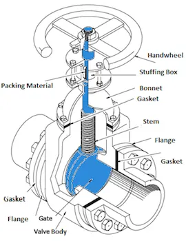
Solving and Modelling Approach –
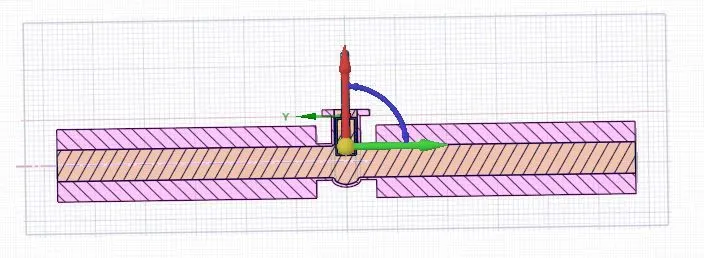
- The Solidworks model of the Gate Valve was imported to Ansys Spaceclaim
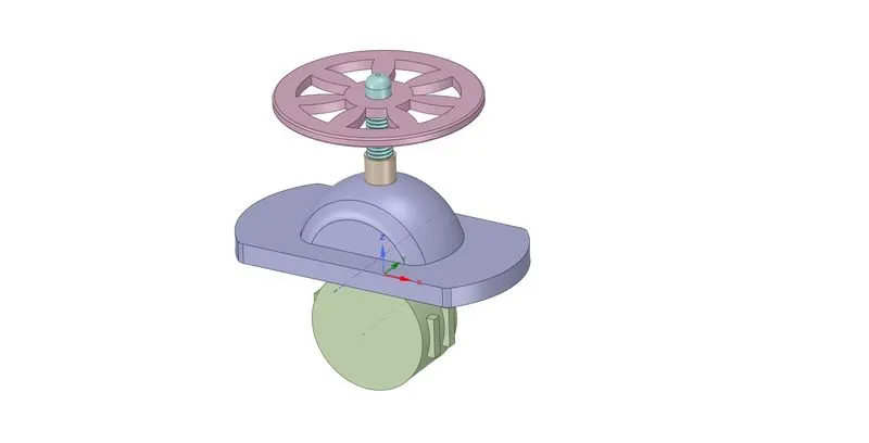
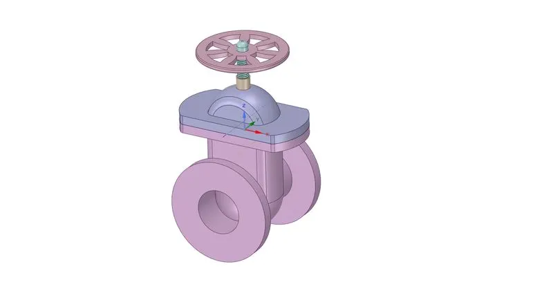
- The Gate Valve consists of mainly 5 components mainly –
- Bottom
- Gate disc
- Bonnet
- Spindle
- Hand wheel
- The fluid volume was extracted from the “prepare” option and edge selection was used to create the fluid volume.
- Then, the gate disc was chosen and the “move” option was selected.
- The gate disc was shifted 10mm in the positive z direction and this was set as the parameter for the parametric study.
- All other components were suppressed and the fluid volume was activated for physics.
- Also, the fluid volume was updated based on context so it can adapt to the rise in level of the gate disc
- The geometry was then further processed for meshing
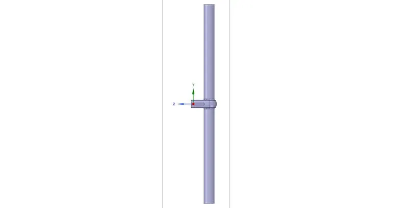
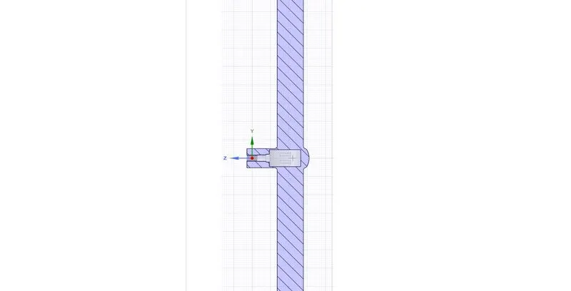
Valve Opening
10mm
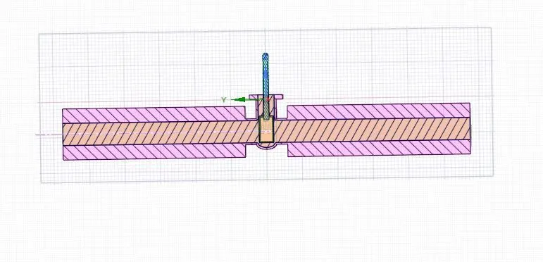
20mm
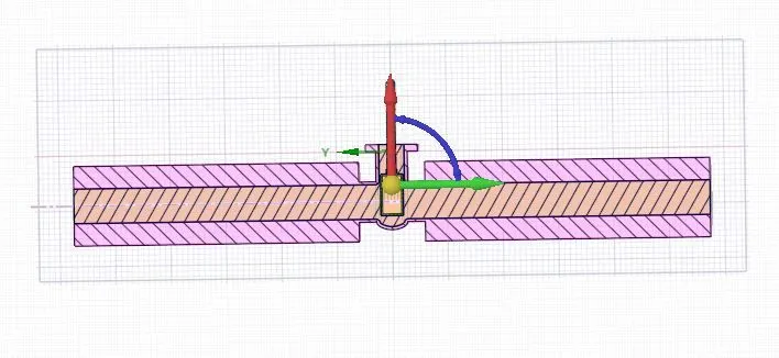
30mm
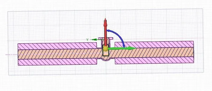
40mm
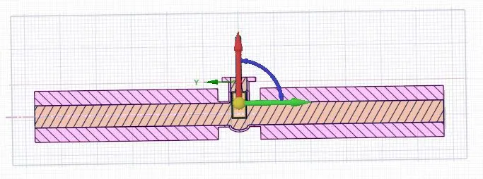
50mm
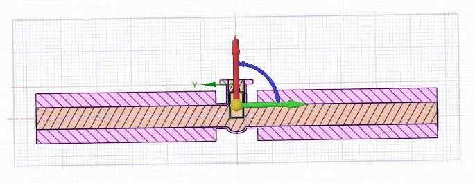
60mm
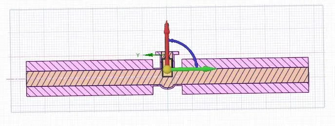
70mm
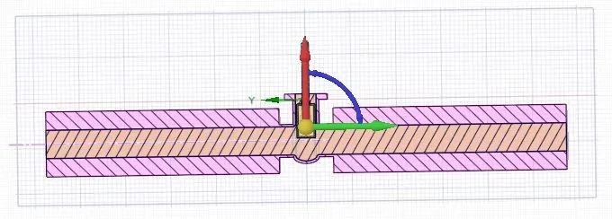
80mm
Meshing –
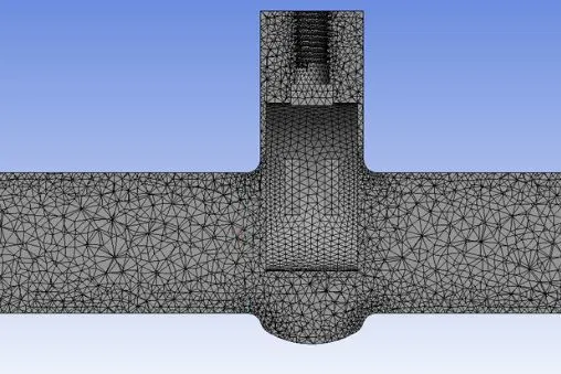
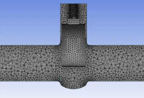
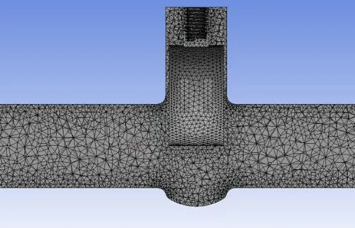
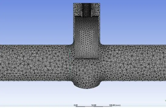
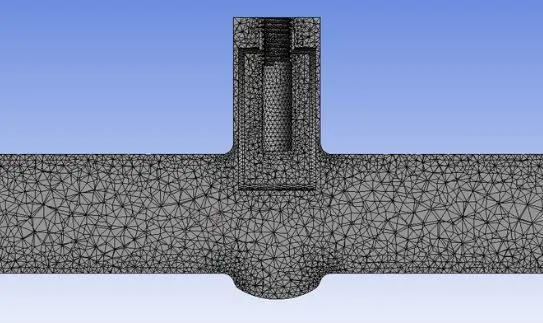
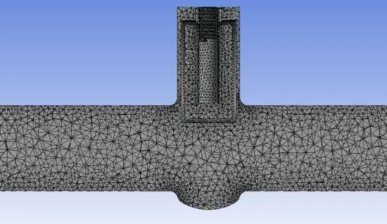
- A standard global meshing was given to the fluid volume.
- Based on the required results, adding inflation layers of refinement to any particular face or body is not necessary.
-
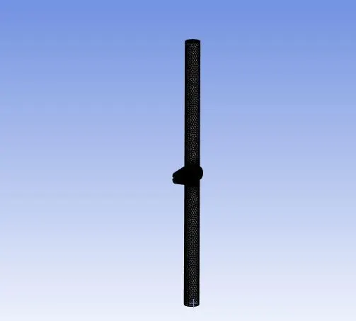
MESH SIZE AS PER VALVE OPENING -
10mm
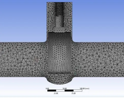
20mm
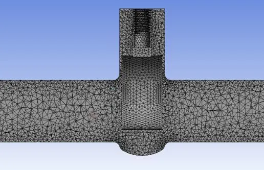
30mm
40mm
50mm
60mm
70mm
80mm
Setting up the case in Ansys Setup –
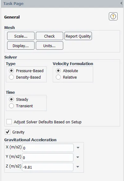
- In this problem, the max velocity attained by water is very less as compared to the speed of sound.
- Hence, the Mach number is <<< 0.3. Hence, a pressure-based solver was used since density-based solvers are generally used for simulations with Mach no > 0.3.
- In this particular simulation, a steady state solver was used since we do not require to observe the properties of the flow at every moment.
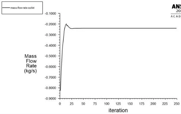
- We only require the values of the final mass flow rate at the outlet.
- Furthermore, a gravity value of 9.81 m/s^2 was added in the -ve Z direction.
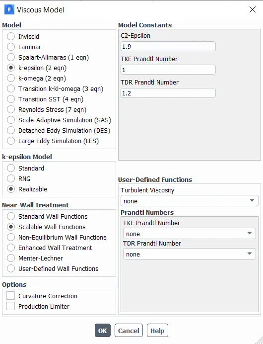
- The k epsilon realizable with scalable wall functions was chosen as the turbulence model for the is particular problem.
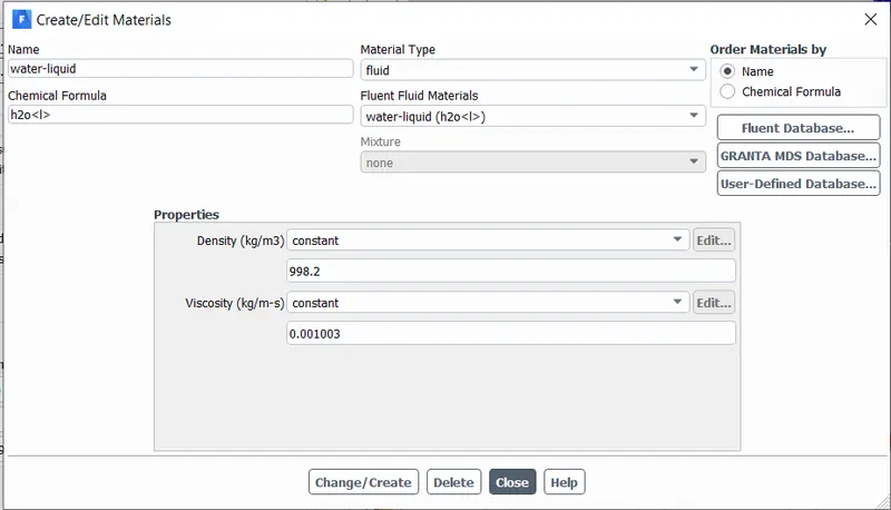
- Furthermore, water-liquid was imported into the ansys fluent materials and air was deleted.
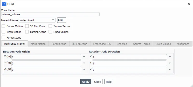
- The cell zone conditions were changed and water-liquid was chosen as the fluid for the computational domain.
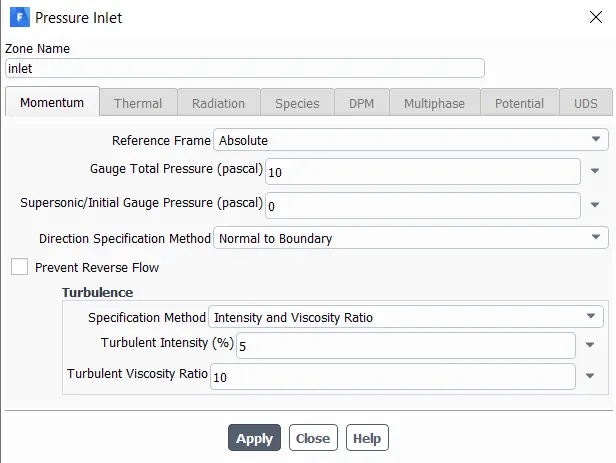
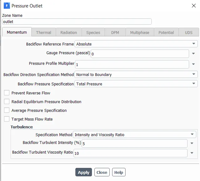
- Afterwards, the boundary conditions were set as follows –
- Inlet – pressure inlet with 10Pa pressure
- Outlet – pressure outlet with 0Pa pressure
- Wall – adiabatic walls
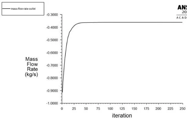
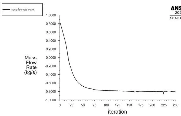
- Report definitions for mass flow rate at the outlet were created and plotted
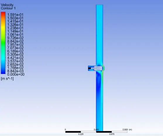
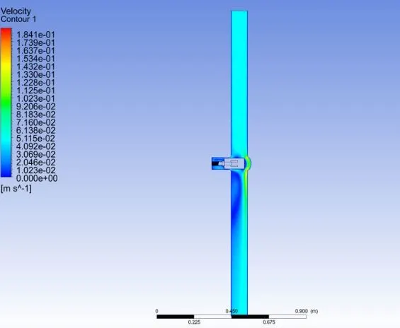
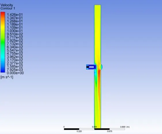
- Similarly, velocity contours and solution animations were generated after initialising the solution
- Standard initialisation with computation from the inlet was done.
- Based on the inlet and outlet pressure, the inlet velocity came out to be -0.1415488m/s in the y direction.
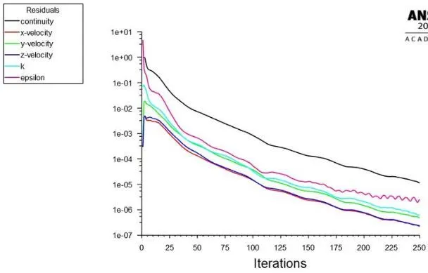
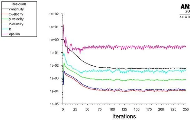
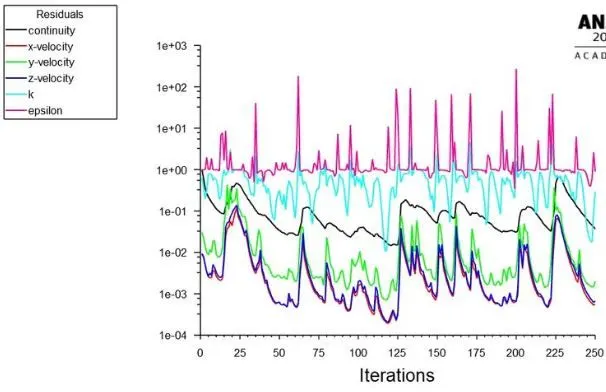
- The simulation was then run for 250 iterations.
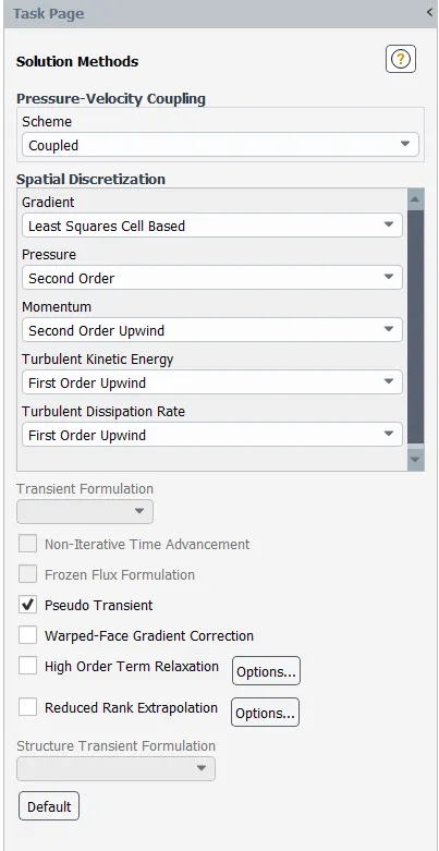
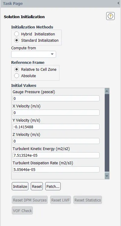
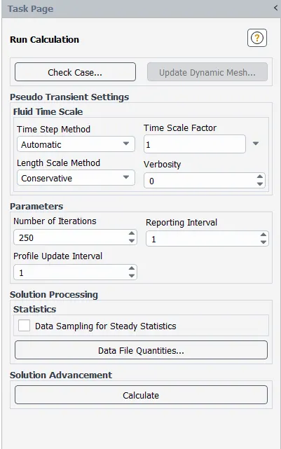
Parametric Study settings –
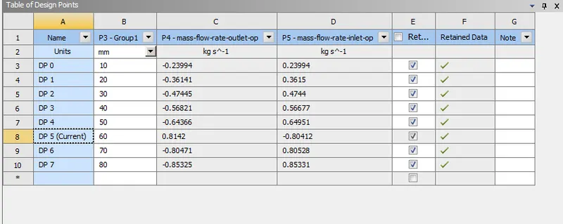
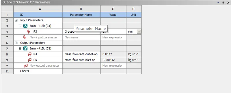
- After completing the 1st iteration, the parametric study tab was opened and design points were added.
- This study was analysed at a Valve opening of 10mm to 80mm in intervals of 10mm.
- Retain data option was chosen so we can observe the contours and plots of each iteration.
- Then “update all design points” was chosen and all the iterations were simulated.
- We can right click on each option and chose “set as current” to analyse the results of that particular iteration.
Results and Findings –
- 10mm
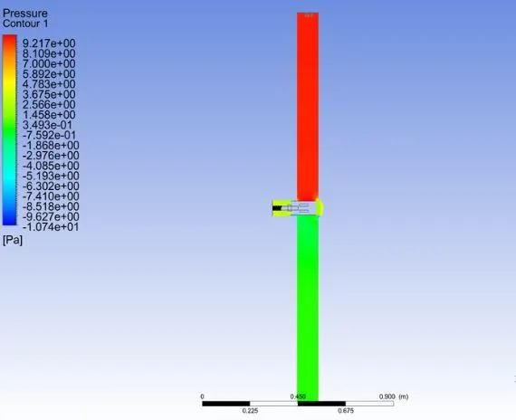
- 20mm
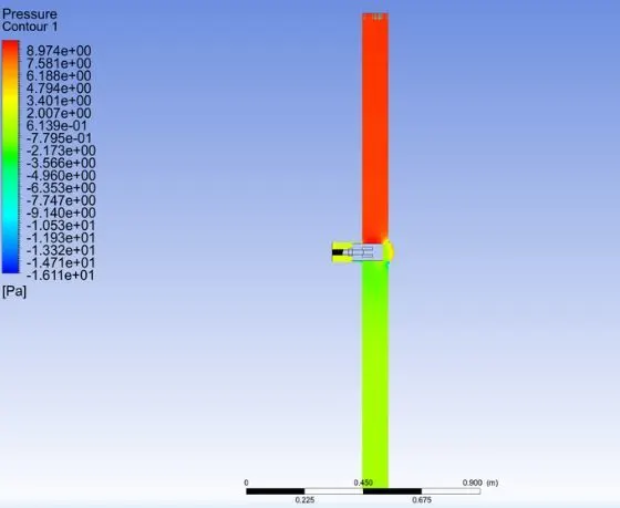
- 30mm
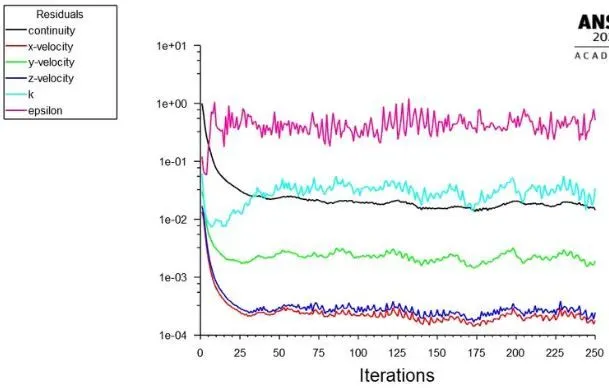
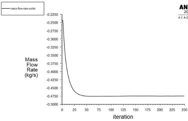
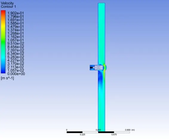
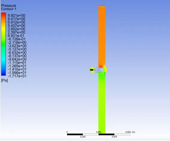
- 40mm
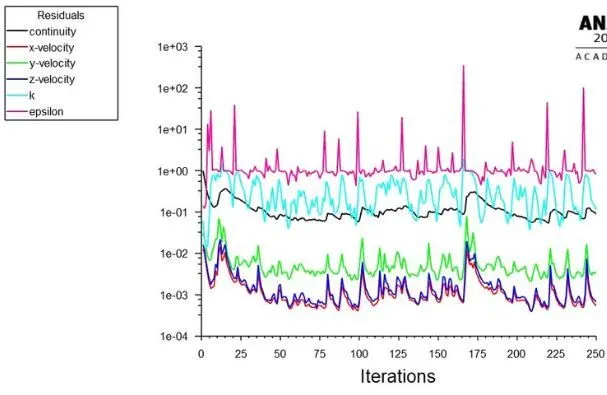
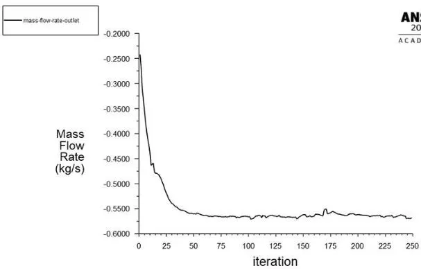
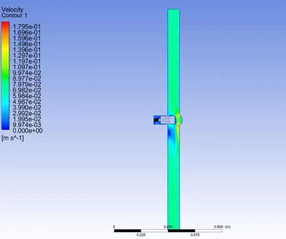
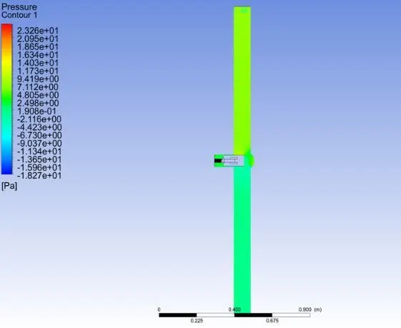
- 50mm
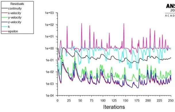
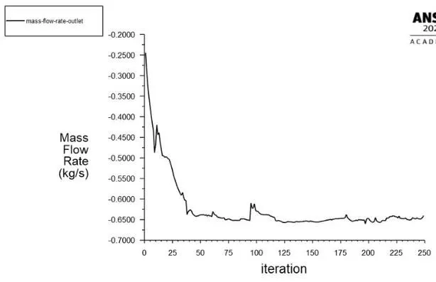
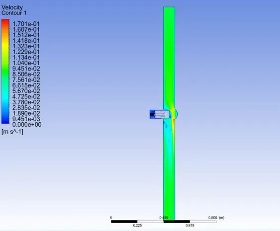
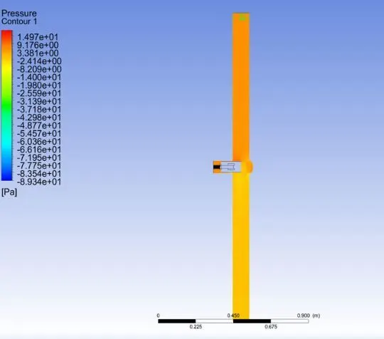
6. 60 mm
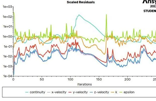
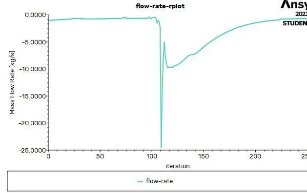
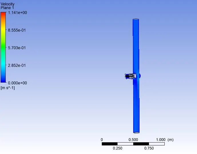
- 70mm
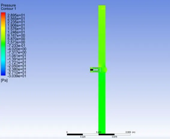
- 80mm
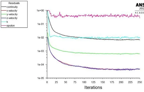
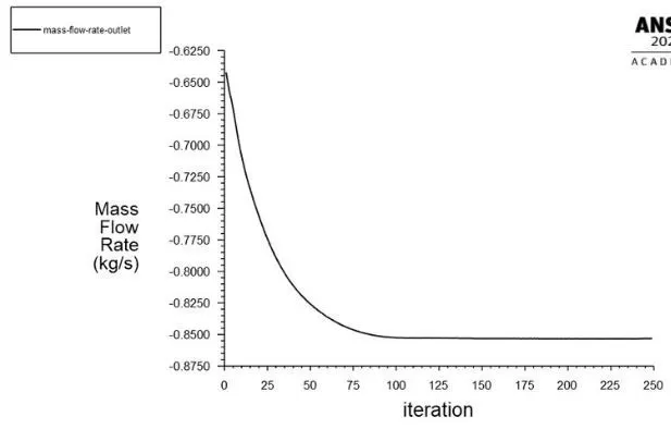
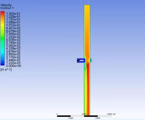
Tables and charts –
Conclusions and inferences –
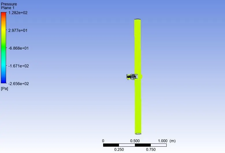
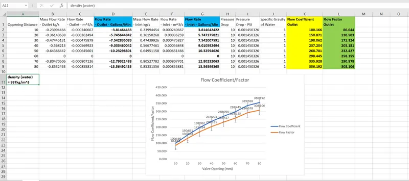
- It can be observed that the mass flow rate at the outlet increases as the opening of the valve increases.
- This is obvious since more openings of the valve will allow more fluid to flow at the same time.
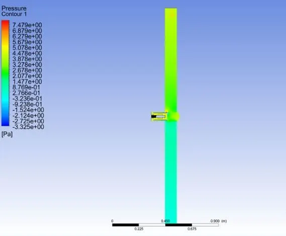
- It can also be observed that as the valve is opened, the pressure difference between the inlet and outlet decreases.
- This can be evident from the pressure contours
- Lastly, the velocity contours smoothen out after increasing the valve opening
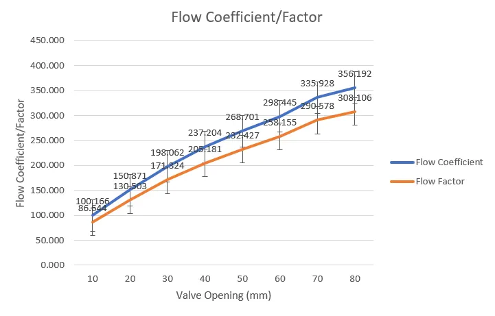
- Last but not the least, the flow factor and flow coefficients increase almost linearly with respect to the valve opening.
- This can be evident from the excel graph as plotted above