Week 7 - Simulation of a 1D Super-sonic nozzle flow simulation using Macormack Method

Aim:

• To simulate the isentropic flow through a 1D quasi subsonic-supersonic nozzle.
• To derive the conservative and non conservative forms of the governing equation and solve them using the MacCormack's technique.
• To determine the steady state the temperature distribution of the flow field variables and investigate the difference between the two forms of governing equations by comparing the solution.

Objective:

• Steady-state of distribution of primitive variables inside the nozzle.
• Time-Wise variation of the primitive variables.
• Variation of mass flow rate distribution inside the nozzle at different time steps during the Time-Marching process.
• Comparision of normalized mass flow rate distribution of both forms.

Theory Explaination:

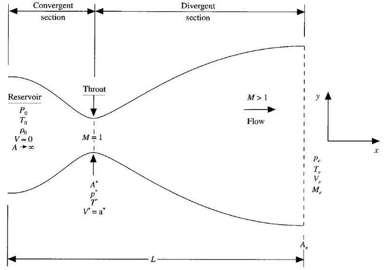
Subsonic-Supersonic nozzle:

Source : Computational fluid dynamics, The basics with applications, J.D Anderson (Book pg. no 285)

The subsonic-supersonic nozzle of length L consists of two sections namely convergent and divergent sections seperated by a throat
region.

Setup:

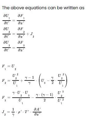
• The governing equation will be explained in the terms of PDE suitable for time-marching solution of quasi 1D flow.
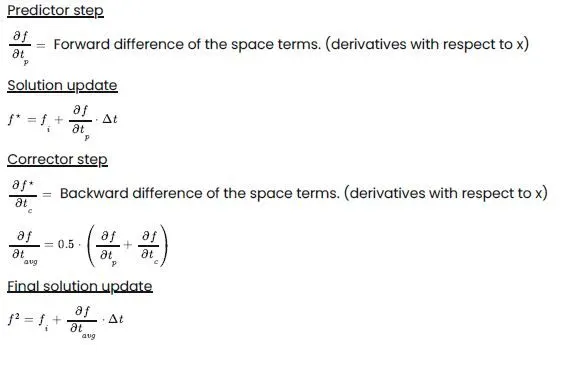
• The finite differencing expressions pertaining to MacCormack's technique will be set up.
• Calcuation of time steps and treatment of initial and boundary conditions will be formulated.

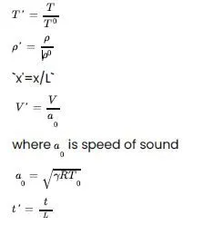
For fluid flow through nozzle, the flow field variables are expressed in non dimensional form. By doing so, the numerical values of these
variables becomes easier to present and compare the results.

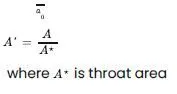
Flow field variables in non dimensional forms:

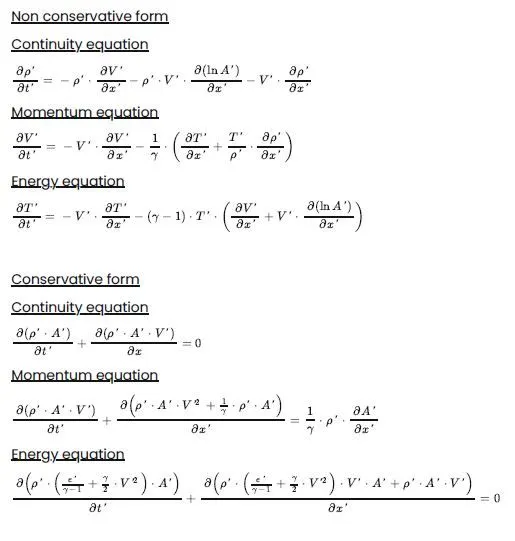
Governing equations (in non dimensional forms):

Meshing:

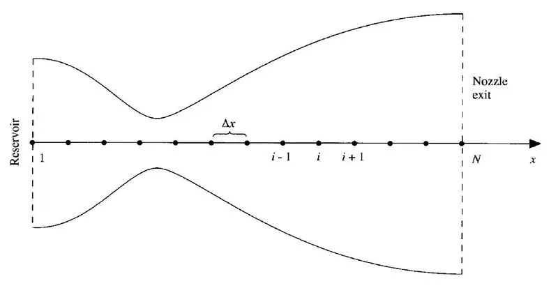
Grid point distribution along the nozzle:

Source : Computational fluid dynamics, The basics with applications, J.D Anderson (Book pg. no 299)

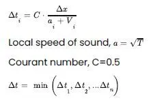
Calculation of time steps:

Discretization:

Boundary Conditions:

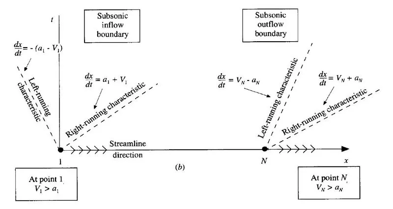
Study of boundary conditions:subsonic inflow and supersonic outflow

Source : Computational fluid dynamics, The basics with applications, J.D Anderson (Book pg. no 304)

Flow is unsteady, inviscid which is governed by hyperbolic equations. For 1D unsteady flow, there exists 2 real characteristic lines for a
point in a plane.

Boundary condition is provided at the domain of dependence.

• If characteristics flows from left to right,Dirichlet boundary conditions is provided which helps to calculate in domain of
  influence. Boundary conditions need to be specified.
• If characteristic lines flow from right to left, Neumann boundary condition is provided which helps to calculate values at the
  boundary by using values at the inner nodes. Boundary conditions need to be floated.

The appropriate initial and boundary conditions for both non-conservative and conservative forms are taken from the Computational
fluid dynamics, The basics with applications, J.D Anderson, textbook.

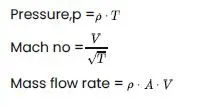
Some important formulas:

MATLAB CODE:

clear all
close all
clc

%inputs
n=31;
x=linspace(0,3,31);
dx=x(2)-x(1);
tic
[t,rho,p,v,mach_no,mass_flow_rate,rho_throat,v_throat,p_throat,t_throat,mach_throat]=non_conservative_form(n,x,dx);
time1=toc;
tic
[t_c,rho_c,p_c,v_c,mach_no_c,mass_flow_rate_c,rho_throat_c,v_throat_c,p_throat_c,t_throat_c,mach_throat_c,dt]=conservative_f
orm(n,x,dx);
time2=toc;

figure(1)
subplot(4,1,1)
plot(x,t,'r','linewidth',1.2)
ylabel('Temperature')
title('Non-conservative form: Distribution of primitive variables along the nozzle length')
subplot(4,1,2)
plot(x,rho,'linewidth',1.2)
ylabel('Density')
subplot(4,1,3)
plot(x,p,'g','linewidth',1.2)
ylabel('Pressure')
subplot(4,1,4)
plot(x,mach_no,'m','linewidth',1.2)
xlabel('Nozzle length')
ylabel('Mach no.')

figure(2)
legend('1st time step','50th time step','100th time step','200th time step','700th time step','1400th time step')
title('Non-conservative form: Variation of Mass flow rate distribution at different time steps')
xlabel('Nozzle length')
ylabel('Mass flow rate')

figure(3)
subplot(4,1,1)
plot(t_throat,'r','linewidth',1.2)
ylabel('Temperature')
title('Non-conservative form: Time-wise variations of primitive variables at throat')
subplot(4,1,2)
plot(rho_throat,'linewidth',1.2)
ylabel('Density')
subplot(4,1,3)
plot(p_throat,'g','linewidth',1.2)
ylabel('Pressure')
subplot(4,1,4)
plot(mach_throat,'m','linewidth',1.2)
xlabel('Time iterations')
ylabel('Mach no.')

figure(4)
subplot(4,1,1)
plot(x,t_c,'r','linewidth',1.2)
ylabel('Temperature')
title('Conservative form: Distribution of primitive variables along the nozzle length')
subplot(4,1,2)
plot(x,rho_c,'linewidth',1.2)
ylabel('Density')
subplot(4,1,3)
plot(x,p_c,'g','linewidth',1.2)
ylabel('Pressure')
subplot(4,1,4)
plot(x,mach_no_c,'m','linewidth',1.2)
xlabel('Nozzle length')
ylabel('Mach no.')

figure(5)
legend('1st time step','50th time step','100th time step','200th time step','700th time step','1400th time step')
title('Conservative form: Variation of Mass flow rate distribution at different time steps')
xlabel('Nozzle length')
ylabel('Mass flow rate')

figure(6)
subplot(4,1,1)
plot(t_throat_c,'r','linewidth',1.2)
ylabel('Temperature')
title('Conservative form: Time-wise variations of primitive variables at throat')
subplot(4,1,2)
plot(rho_throat_c,'linewidth',1.2)
ylabel('Density')
subplot(4,1,3)
plot(p_throat_c,'g','linewidth',1.2)
ylabel('Pressure')
subplot(4,1,4)
plot(mach_throat_c,'m','linewidth',1.2)
xlabel('Time iterations')
ylabel('Mach no.')

figure(7)
plot(x,mass_flow_rate,'linewidth',1.2)
hold on
plot(x,mass_flow_rate_c,'m','linewidth',1.2)
hold on
legend('Non-conservative form','Conservative form')
xlabel('Nozzle length')
ylabel('Mass flow rate')
title(' Comparison of Normalized mass flow rate distributions of both forms')

Function Code:

Non-Conservative form:

function[t,rho,p,v,mach_no,mass_flow_rate,rho_throat,v_throat,p_throat,t_throat,mach_throat]=non_conservative_form(n,x,dx)

%Initial profiles
rho=1-0.3146*x;
t=1-0.2314*x;
v=(0.1+1.09*x).*(t).^0.5;
gamma=1.4;

%area
a=1+2.2*(x-1.5).^2;
%time steps
nt=1400;
dt=min(0.5*dx./(v+sqrt(t)));

%Outer time step
for k=1:nt
% Copy of variables
rho_old=rho;
v_old=v;
t_old=t;

%Predictor method
for j=2:n-1
dvdx=(v(j+1)-v(j))/dx;
drhodx=(rho(j+1)-rho(j))/dx;
dtdx=(t(j+1)-t(j))/dx;
dlogadx=(log(a(j+1))-log(a(j)))/dx;

%Contuinity equation
drhodt_p(j)=-rho(j)*dvdx-rho(j)*v(j)*dlogadx-v(j)*drhodx;

%Momentum equation
dvdt_p(j)=-v(j)*dvdx-(1/gamma)*(dtdx+(t(j)/rho(j))*drhodx);

%Energy equation
dtdt_p(j)=-v(j)*dtdx-(gamma-1)*t(j)*((dvdx+v(j)*dlogadx));

%Solution update
rho(j)=rho(j)+drhodt_p(j)*dt;
v(j)=v(j)+dvdt_p(j)*dt;
t(j)=t(j)+dtdt_p(j)*dt;
end

%Corrector method
for j=2:n-1
  dvdx=(v(j)-v(j-1))/dx;
  drhodx=(rho(j)-rho(j-1))/dx;
  dtdx=(t(j)-t(j-1))/dx;
  dlogadx=(log(a(j))-log(a(j-1)))/dx;

  %Contuinity equation
  drhodt_c(j)=-rho(j)*dvdx-rho(j)*v(j)*dlogadx-v(j)*drhodx;
  %Momentum equation
  dvdt_c(j)=-v(j)*dvdx-(1/gamma)*(dtdx+(t(j)/rho(j))*drhodx);
  %Energy equation
  dtdt_c(j)=-v(j)*dtdx-(gamma-1)*t(j)*((dvdx+v(j)*dlogadx));
end

%Average time derivative
drhodt=0.5*(drhodt_p+drhodt_c);
dvdt=0.5*(dvdt_p+dvdt_c);
dtdt=0.5*(dtdt_p+dtdt_c);
% Final Solution update
for i=2:n-1
 rho(i)=rho old(i)+drhodt(i)*dt;

  v(i)=v_old(i)+dvdt(i)*dt;
  t(i)=t_old(i)+dtdt(i)*dt;
end

%Boundary conditions
%Inlet
v(1)=2*v(2)-v(3);
%Outlet
v(n)=2*v(n-1)-v(n-2);
rho(n)=2*rho(n-1)-rho(n-2);
t(n)=2*t(n-1)-t(n-2);

%Calculation of pressure, mach number and mass flow rate
p=rho.*t;
mach_no=v./sqrt(t);
mass_flow_rate=rho.*a.*v;

%Calculation of pressure, mach number and mass flow rate at throat
p_throat(k) = p(16);
v_throat(k) = v(16);
mach_throat(k) = mach_no(16);
t_throat(k) = t(16);
rho_throat(k) = rho(16);

%Variation of Mass flow rate distribution inside the nozzle at different time steps
figure(2)
   if k==1
   plot(x,mass_flow_rate,'linewidth',1.2)
   hold on
   elseif k==50
   plot(x,mass_flow_rate,'cyan','linewidth',1.2)
   hold on
   elseif k==100
   plot(x,mass_flow_rate,'r','linewidth',1.2)
   hold on
   elseif k==200
   plot(x,mass_flow_rate,'m','linewidth',1.2)
   hold on
   elseif k==700
   plot(x,mass_flow_rate,'k','linewidth',1.2)
   hold on
   elseif k==1400
   plot(x,mass_flow_rate,'*g','linewidth',1.2)
   hold on
   end
  end
end

Conservative form:

function[t_c,rho_c,p_c,v_c,mach_no_c,mass_flow_rate_c,rho_throat_c,v_throat_c,p_throat_c,t_throat_c,mach_throat_c,dt]=conservative_form(n,x,dx)

% Initial profiles
for i=1:n
   if (0<=x(i) && x(i)<=0.5)
   rho_c(i)=1;
   t_c(i)=1;
   elseif (0.5<=x(i) && x(i)<=1.5)
   rho_c(i)=1-0.366*(x(i)-0.5);
   t_c(i)=1-0.167*(x(i)-0.5);
   elseif (1.5<=x(i) && x(i)<=3.5)
   rho_c(i)=0.634-0.3879*(x(i)-1.5);
   t_c(i)=0.833-0.3507*(x(i)-1.5);
   end
end

%area
a=1+2.2*(x-1.5).^2;
gamma=1.4;
v_c=0.59./(rho_c.*a);

% Solutions vectors
u1=rho_c.*a;
u2=rho_c.*a.*v_c;
u3=rho_c.*(t_c/(gamma-1)+(gamma/2)*v_c.^2).*a;

%time steps
nt=1400;
dt=min(0.5*dx./(v_c+sqrt(t_c)));

%Outer time step
   for k=1:nt
   % Copy of values of u1,u2,u3
   u1_old=u1;
   u2_old=u2;
   u3_old=u3;
   %Flux vectors
   f1=u2;
   f2=(u2).^2./u1+((gamma-1)/gamma)*(u3-(gamma/2)*((u2).^2./u1));
   f3=(gamma*u2.*u3)./u1-((gamma*(gamma-1)))/2*((u2).^3./(u1).^2);
   %Predictor method
   for j=2:n-1
    j2=(1/gamma)*rho_c(j)*t_c(j)*((a(j+1)-a(j))/dx);
  %Contuinity equation
  du1dt_p(j)=-(f1(j+1)-f1(j))/dx;
  %Momentum equation
  du2dt_p(j)=(-(f2(j+1)-f2(j))/dx)+j2;
  %Energy equation
  du3dt_p(j)=-(f3(j+1)-f3(j))/dx;
  %Solution update
  u1(j)=u1(j)+du1dt_p(j)*dt;
  u2(j)=u2(j)+du2dt_p(j)*dt;
  u3(j)=u3(j)+du3dt_p(j)*dt;
end

%Updating primitive variables
rho_c=u1./a;
t_c=(gamma-1)*((u3)./(u1)-(gamma/2)*((u2)./(u1)).^2);
%Updating Flux vectors

f1=u2;
f2=(u2).^2./u1+((gamma-1)/gamma)*(u3-(gamma/2)*((u2).^2./u1));
f3=(gamma*u2.*u3)./u1-(gamma*(gamma-1))/2*((u2).^3./(u1).^2);

%Corrector method
for j=2:n-1
j2=(1/gamma)*rho_c(j)*t_c(j)*((a(j)-a(j-1))/dx);

%Contuinity equation
du1dt_c(j)=-(f1(j)-f1(j-1))/dx;

%Momentum equation
du2dt_c(j)=-((f2(j)-f2(j-1))/dx)+j2;
%Energy equation
du3dt_c(j)=-(f3(j)-f3(j-1))/dx;
end

%Average time derivative
du1dt=0.5*(du1dt_p+du1dt_c);
du2dt=0.5*(du2dt_p+du2dt_c);
du3dt=0.5*(du3dt_p+du3dt_c);

% Final Solution update
for m=2:n-1
u1(m)=u1_old(m)+du1dt(m)*dt;
u2(m)=u2_old(m)+du2dt(m)*dt;
u3(m)=u3_old(m)+du3dt(m)*dt;
end

%Boundary conditions
%Inlet
u1(1)=a(1);
u2(1)=2*u2(2)-u2(3);
u3(1)=u1(1)*(t_c(1)/(gamma-1)+(gamma/2)*(v_c(1))^2);
%Outlet
u1(n)=2*u1(n-1)-u1(n-2);
u2(n)=2*u2(n-1)-u2(n-2);
u3(n)=2*u3(n-1)-u3(n-2);

% Final update of primitive variables
rho_c=u1./a;
t_c=(gamma-1)*((u3)./(u1)-(gamma/2)*((u2)./(u1)).^2);
v_c=(u2)./(u1);

%Calculation of pressure, mach number and mass flow rate
p_c=rho_c.*t_c;
mach_no_c=v_c./sqrt(t_c);
mass_flow_rate_c=rho_c.*a.*v_c;

%Calculation of pressure, mach number and mass flow rate at throat
p_throat_c(k) = p_c(16);
v_throat_c(k) = v_c(16);
mach_throat_c(k) = mach_no_c(16);
t_throat_c(k) = t_c(16);
rho_throat_c(k) = rho_c(16);

%Variation of Mass flow rate distribution inside the nozzle at different time steps

figure(5)
  if k==1
  plot(x,mass_flow_rate_c,'linewidth',1.2)
  hold on
  elseif k==50
  plot(x,mass_flow_rate_c,'cyan','linewidth',1.2)
  hold on
  elseif k==100
  plot(x,mass_flow_rate_c,'r','linewidth',1.2)
  hold on
  elseif k==200

   plot(x,mass_flow_rate_c,'m','linewidth',1.2)
   hold on
   elseif k==700
   plot(x,mass_flow_rate_c,'k','linewidth',1.2)
   hold on
   elseif k==1400
   plot(x,mass_flow_rate_c,'*g','linewidth',1.2)
   hold on
   end
  end
end

Explanation
Initially the grid size (n), x and dx values are assigned.
Then the function non-conservation form is executed. Under the function, the initial profiles (rho, T, V), area of nozzle, time step values are assigned.
Loop for outer time step is initiated under which the copy of variables (rho, T, V) is created and the McCormack’s method is carried out.
Predictor method followed by solution update is done. Corrector method followed by final solution update is also done.
The boundary conditions at the inlet and outlet are given. Then pressure, mach no. and mass flow rate are calculated.
The values of primitive variables at the throat are assigned to variables with size k so that for each timestep, the values at throat are calculated.
Then the mass flow rates at different time steps are plotted.
The above process is repeated for 1400-time steps and the function returns the final values of primitive variables to the main program.
Then the function conservation form is executed. The same process as followed in non-conservation form is repeated except that flux vectors (F1, F2, F3) and solutions vectors (U1, U2, U3) are used in this form.
In McCormack’s method, the flux vectors and solutions vectors are used and then primitive variables are updated.
The above process is repeated for 1400-time steps and the function returns the final values of primitive variables to the main program.
The simulation time for the conservation form and non-conservation form are stored in variables time1, time2 respectively.
Then finally the respective plots are obtained using figure and subplot commands.

Output
The primitive variables, mass flow rate along x-axis and the nozzle length along y-axis, all are in non-dimensional form in all the plots.
Non conservative form
Figure 1

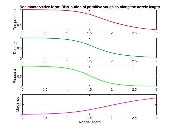
figure 2:

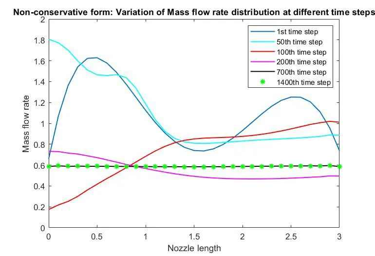
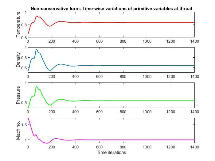
figure 3

Explanation
In figure 1, the temperature, density and pressure values decrease as the nozzle length increases. But mach no increases as nozzle length increases.
In figure 2, the mass flow rates at time steps are plotted. It can be seen that for 700 and 1400 timesteps the mass flow rate does not change as nozzle length increases. So, we can say that it has almost reached steady state around 700 time step.
In figure 3, there are some fluctuations in primitive variables at the initial time iterations and then the plots become linear which implies that they attained steady states.

conservative form:

figure 4:

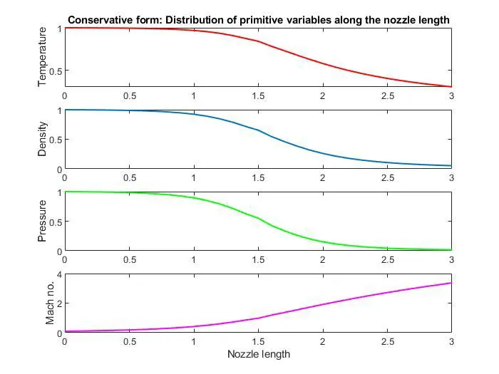
figure 5

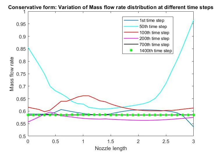
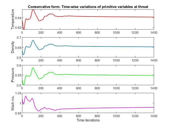
figure 6

Explanation:

In figure 4, the temperature, density and pressure values decrease as the nozzle length increases. But mach no. increases as nozzle length increases.
In figure 5, the mass flow rates at time steps are plotted. It can be seen that for 700 and 1400 timesteps the mass flow rate does not change as nozzle length increases. So, we can say that it has almost reached steady state around 700 time step.
In figure 6, there are some fluctuations in primitive variables at the initial time iterations and then the plots become linear which implies that they attained steady states.

Comparision of mass flow rates:

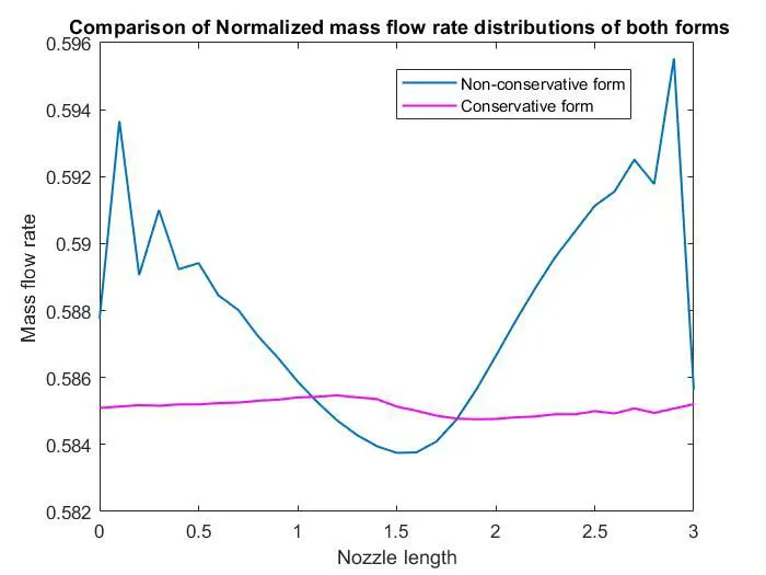
figure 7

Explanation
In figure 7, it is seen that conservation form yields the better mass flow distribution than non-conservation form.

Grid independence test:

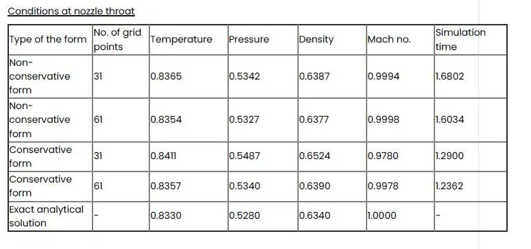
When the grid size,n=31, the values of the primitive variables at the throat region of the nozzle is given in the table below. On doubling
the grid size say n=61, we get the primitive variable values almost same as we got for grid size n=31 for non conservative form. The
same applies to the conservative form as well. The values of both non-conservative and conservative forms are almost closer to the
exact analytical solution. So the change in grid size does not have much impact on values of primitive variables for both the forms.
So the calculations done using non-conservative and conservative forms are grid independent.

Observations
The conservation form does a better job in conserving the mass flow than the non-conservation form.
The solution of conservation form requires more work and calculational effort as it involves flux variables and solutions vectors.
In non-conservation form, not much work is required as primitive variables are directly used for calculation.
Simulation time of conservation form is lesser than that of non-conservation form. So, the convergence rate is faster in conservation form.

Conclusion
Using MATLAB, the isentropic flow through a quasi 1D subsonic-supersonic nozzle was simulated.
The conservation and non-conservation forms of the governing equations were solved using McCormack’s technique.
Distribution of primitive variables, mass flow rate through the nozzle and time-wise variations of primitive variables at throat were plotted for both of the forms.
Both conservation and non-conservation forms were found to be grid independent.