Week 5.1 - Mid term project - Solving the steady and unsteady 2D heat conduction problem

Objective:

Solve the 2D heat conduction equation by using the point iterative techniques
1. Jacobi
2. Gauss-seidel
3. Successive over-relaxation.

Your absolute error criteria is 1e-4

1.Steady state analysis
2.Transient state analysis using explicit and implicit schemes.

code:

close all
clear all
clc

nx = 10; %nx & ny will be nodes along the length of x & y respectively
ny = nx; %let us consider nx = ny
x = linspace(0,1,nx); %to create nx number of points from origin to length of domain =1
y = linspace(0,1,ny); %to create ny number of points from origin to length of domain =1

dx=(x(2)-x(1));
dy=(y(2)-y(1));
k=2* (dx^2 + dy^2)/(dx^2 * dy^2);

%let us consider the boundary conditions
top=600;
bottom=900;
left=400;
right=800;

%let us start by taking all values as ones - nx rows and ny columns
T = ones(nx,ny);

%assiging those boundary conditions to the T matrix excepting the corners
T(1,2:nx-1) = top; %to assign the values for first row of T matrix
T(ny,2:nx-1) = bottom; %to assign the values for last row of T matrix
T(2:ny-1,1) = left; %to assign the values for first column of T matrix
T(2:ny-1,nx) = right; %to assign the values for last column of T matrix

%assigning the values at the corner positions of the T matrix by taking average of adjacent values
T(1,1)=(top+left)/2;
T(ny,1)=(bottom+left)/2;
T(1,nx)=(right+top)/2;
T(ny,nx)=(right+bottom)/2;

%dummy variables are created for updating the values
%T & Told are used for jacobi method
%Told1 & Told2 are used for Gauss-seidel method
%Told3 & Told4 are used for SOR method
Told=T;
Told1=T;
Told2=T;
Told3=T;
Told4=T;

%assigining the error value for each method
error_jacobi = 9e9;
tolerance = 1e-4;

%every method should be strted with iteration number 1
j_iter=1;

%for SOR method
alpha=1.5; %alpha should be between 0 & 2

%jacobi method========================================================================
tic
while (error_jacobi > tolerance)
  for i = 2:nx-1 %space loop
   for j = 2:ny-1
       T(i,j) = 1/k * ((Told(i+1,j)+Told(i-1,j))/dx^2+(Told(i,j+1)+Told(i,j-1))/dy^2);
    end
  end
   error_jacobi = max(max(abs(Told-T)));
   Told = T;
   j_iter = 1+j_iter;
end
a=toc;
fprintf('Computational time using Jacobi method = %g n',a);
fprintf('No. of iterations in Jacobi method = %d n',j_iter);
figure(1)
     contourf(T); %to get output as contour
     colormap(jet); %color of contour to get rainbow colors
     colorbar; %side bar representing the temperature with color
     title_text = sprintf('No. of iterations in Jacobi method = %d',j_iter); %to show the iteration number
     title(title_text); %title of plot
     set(gca, 'YDir','reverse')

Gauss sidal method===========================================================

GS_iter=1;

tic
  while (error_gauss > tolerance)
    for i = 2:nx-1
     for j = 2:ny-1
         Told1(i,j) = ((Told1(i+1,j)+Told1(i-1,j))/dx^2+(Told1(i,j+1)+Told1(i,j-1))/dy^2)/k;
     end
   end
    error_gauss = max(max(abs(Told2-Told1)));
    Told2 = Told1;
    GS_iter = GS_iter+1;
end

b=toc;
fprintf(' nComputational time using Gauss-seidel method = %g n',b);
fprintf('No. of iterations in Gauss-seidel method = %d n',GS_iter);
figure(2)
    contourf(Told1);
    colormap(jet);
    colorbar;
    title_text = sprintf('No. of iterations in Gauss-seidel method = %d',GS_iter);
    title(title_text);
    set(gca, 'YDir','reverse')

SOR Method================================================================

%every method should be strted with iteration number 1
SOR_iter=1;

%for SOR method
alpha=1.5; %alpha should be between 0 & 2

%SOR method
tic
   while (error_SOR > tolerance)
     for i = 2:nx-1
      for j = 2:ny-1
          Told3(i,j) = (1-alpha)*Told4(i,j)+(alpha/k)*((Told3(i+1,j)+Told3(i-1,j))/dx^2+
          (Told3(i,j+1)+Told3(i,j-1))/dy^2);
      end
    end
    error_SOR = max(max(abs(Told4-Told3)));
    Told4 = Told3;
    SOR_iter = SOR_iter+1 ;
end

c=toc;
fprintf(' nComputational time using SOR method = %g n',c);
fprintf('No. of iterations in SOR method = %d n',SOR_iter);
figure(3)
     contourf(Told3);
     colormap(jet);
     colorbar;
     title_text = sprintf('No. of iterations in SOR method = %d',SOR_iter);
     title(title_text);
     set(gca, 'YDir','reverse')

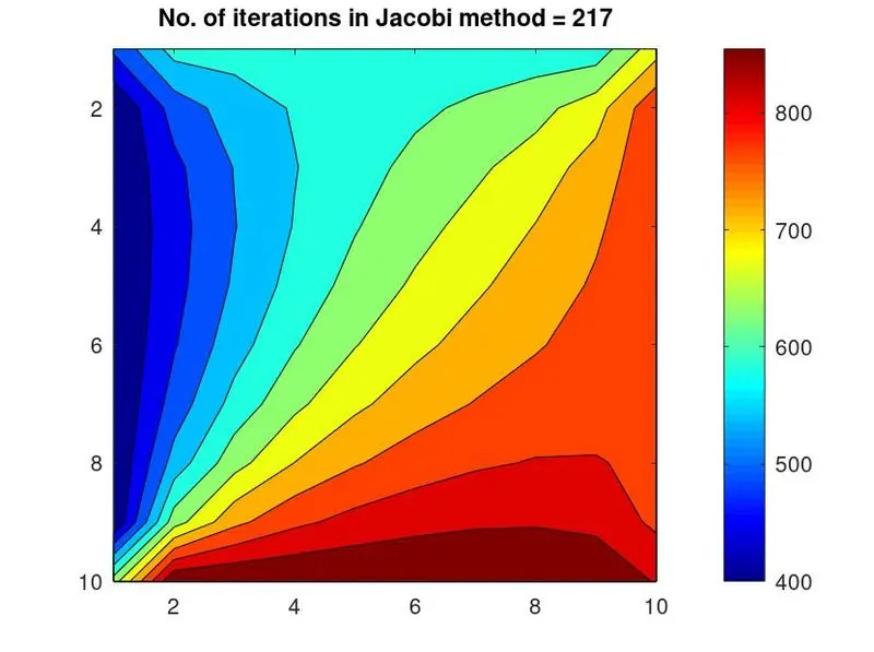
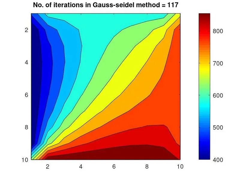
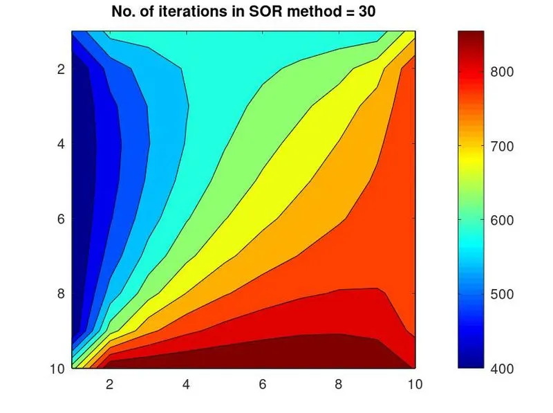
Results:

explicit sheme============================================================

code:

close all
clear all
clc

nx = 20; %nx & ny will be nodes along the length of x & y respectively
ny = nx; %let us consider nx = ny
x = linspace(0,1,nx); %to create nx number of points from origin to length of domain =1
y = linspace(0,1,ny); %to create ny number of points from origin to length of domain =1
dx=(x(2)-x(1));
dy=(y(2)-y(1));
thermal_diffusivity = 1.3;
dt = 4e-4;
time=5;
cfl = 2*thermal_diffusivity*(dt/dx^2);
k1 = thermal_diffusivity*dt/dx^2;
k2 = thermal_diffusivity*dt/dy^2;
nt = time/dt;

%let us consider the boundary conditions
top=600;
bottom=900;
left=400;
right=800;

%let us start by taking all values as ones - nx rows and ny columns
Tfirst = ones(nx,ny);

%assiging those boundary conditions to the T matrix excepting the corners
Tfirst(1,2:nx-1) = top; %to assign the values for first row of T matrix
Tfirst(ny,2:nx-1) = bottom; %to assign the values for last row of T matrix
Tfirst(2:ny-1,1) = left; %to assign the values for first column of T matrix
Tfirst(2:ny-1,nx) = right; %to assign the values for last column of T matrix

%assigning the values at the corner positions of the T matrix by taking average of adjacent values
Tfirst(1,1)=(top+left)/2;
Tfirst(ny,1)=(bottom+left)/2;
Tfirst(1,nx)=(right+top)/2;
Tfirst(ny,nx)=(right+bottom)/2;

%dummy variables are created for updating the values
Tprev = Tfirst;
Tnew = Tfirst;

%every method should be strted with iteration number 1
plane_iter = 1;

term1 = (1-(2*k1)-(2*k2));
tolerance=1e-4;

%transient state - explicit scheme
tic
    for t=1:nt
        error = 9e9;%time loop
         for i = 2:nx-1 %space loop
         for j = 2:ny-1
             H1=k1*(Tprev(i+1,j)+Tprev(i-1,j));
             V1=k2*(Tprev(i,j+1)+Tprev(i,j-1));
             Tnew(i,j) = (term1*Tprev(i,j))+(H1)+(V1);
         end
       end
         error = max(max(abs(Tprev-Tnew)));
         Tprev = Tnew;
         plane_iter = 1+plane_iter;
      if error==0; % to stop the loop after reaching convergence
         break
      end
 end
a=toc;
fprintf(' nComputational time using Explicit method = %g n',a);
fprintf('No. of time levels approached in explicit method = %d n',plane_iter);
figure(1)
     contourf(Tnew); %to get output as contour
     colormap(jet); %color of contour to get rainbow colors
     colorbar; %side bar representing the temperature with color
     title_text = sprintf('No. of time levels approached in explicit scheme to get final output = %g',plane_iter ); %to show the time loop number
     title(title_text) %title of plot
     set(gca, 'YDir','reverse')   

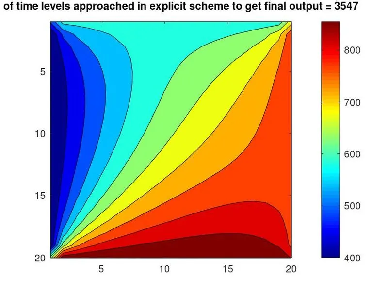
Result:

Conclusion:

From the above figure,the solution is converged at 3547 level

Implicit scheme======================================================

code:

close all
clear all
clc

nx = 20; %nx & ny will be nodes along the length of x & y respectively
ny = nx; %let us consider nx = ny
x = linspace(0,1,nx); %to create nx number of points from origin to length of domain =1
y = linspace(0,1,ny); %to create ny number of points from origin to length of domain =1
dx=(x(2)-x(1));
dy=(y(2)-y(1));
thermal_diffusity = 1.4;
dt = 4e-4;
time=5;
k1 = thermal_diffusity*dt/dx^2;
k2 = thermal_diffusity*dt/dy^2;
nt = time/dt;

%let us consider the boundary conditions
top=600;
bottom=900;
left=400;
right=800;

%let us start by taking all values as ones - nx rows and ny columns
T = ones(nx,ny);

%assiging those boundary conditions to the T matrix excepting the corners
T(1,2:nx-1) = top; %to assign the values for first row of T matrix
T(ny,2:nx-1) = bottom; %to assign the values for last row of T matrix
T(2:ny-1,1) = left; %to assign the values for first column of T matrix
T(2:ny-1,nx) = right; %to assign the values for last column of T matrix

%assigning the values at the corner positions of the T matrix by taking average of adjacent values
T(1,1)=(top+left)/2;
T(ny,1)=(bottom+left)/2;
T(1,nx)=(right+top)/2;
T(ny,nx)=(right+bottom)/2;
term1 = 1/(1+2*k1+2*k2);
term2 = k1* term1;
term3 = k2* term1;

%dummy variables are created for updating the values of next time step
Tprev1=T; %for jacobi
Tprev2=T; %for Gauss-seidel
Tprev3=T; %for SOR

%dummy variables are created for updating the values
%T & Told are used for jacobi method
%Told1 & Told2 are used for Gauss-seidel method
%Told3 & Told4 are used for SOR method
Told=T;
Told1=T;
Told2=T;
Told3=T;
Told4=T;
tolerance = 1e-4;

%every method should be strted with iteration number 1
j_iter=1;
GS_iter=1;
SOR_iter=1;

%every method should be strted with 1st time loop
j_time=1;
GS_time=1;
SOR_time=1;

%for SOR method
alpha=1.2; %alpha should be between 1 & 2
k=2* (dx^2 + dy^2)/(dx^2 * dy^2);

%jacobi method - transient state - implicit scheme
tic
  for t=1:nt %time loop
     error_jacobi = 9e9;
      while (error_jacobi > tolerance)
       for i = 2:nx-1 %space loop
        for j = 2:ny-1
            H1 = Told(i+1,j)+Told(i-1,j);
            V1 = Told(i,j+1)+Told(i,j-1);
            T(i,j) = (term1*Tprev1(i,j))+(term2*H1)+(term3*V1);
       end
     end
      error_jacobi= max(max(abs(Told-T)));
      Told= T;
      j_iter = 1+j_iter;
   end
    Tprev1=T;
    j_time=1+j_time;
   if (error_jacobi==0)
    break
  end
end

a=toc;
fprintf(' nComputational time using implicit Jacobi method = %g n',a);
fprintf('No. of iterations in implicit Jacobi method = %d n',j_iter);
fprintf('No. of time levels approached in implicit Jacobi method = %d n',j_time);
figure(1)
       contourf(T); %to get output as contour
       colormap(jet); %color of contour to get rainbow colors
       colorbar; %side bar representing the temperature with color
       title_text = sprintf('No. of iterations using jacobi in implicit-transient=%d, No. of time levels=%g',j_iter,j_time); %to show the iteration number
       title(title_text) %title of plot
       set(gca, 'YDir','reverse')

%Gauss_seidel method - transient state - implicit scheme
tic
    for t=1:nt %time loop
        error_gauss = 9e9;
      while (error_gauss > tolerance)
       for i = 2:nx-1 %space loop
        for j = 2:ny-1
           H2 = Told2(i+1,j)+Told1(i-1,j);
           V2 = Told2(i,j+1)+Told1(i,j-1);
           Told1(i,j) = (term1*Tprev2(i,j))+(term2*H2)+(term3*V2);
        end
      end
      error_gauss= max(max(abs(Told2-Told1)));
      Told2= Told1;
      GS_iter = 1+GS_iter;
end
Tprev2=Told2;
GS_time=1+GS_time;
   if (error_gauss==0)
     break
   end
end

b=toc;
fprintf(' nComputational time using implicit GS method = %g n',b);
fprintf('No. of iterations in implicit GS method = %d n',GS_iter);
fprintf('No. of time levels approached in implicit GS method = %d n',GS_time);
figure(2)
      contourf(Told1); %to get output as contour
      colormap(jet); %color of contour to get rainbow colors
      colorbar; %side bar representing the temperature with color
      title_text = sprintf('No. of iterations using Gauss-seidel in implicit-transient=%d, No. of time levels=%g',GS_iter,GS_time); %to show the iteration number
      title(title_text) %title of plot
      set(gca, 'YDir','reverse')

%SOR method - transient state - implicit scheme
tic
   for t=1:nt %time loop
       error_SOR = 9e9;
     while (error_SOR > tolerance)
      for i = 2:nx-1 %space loop
       for j = 2:ny-1
          H3 = Told4(i+1,j)+Told3(i-1,j);
          V3 = Told4(i,j+1)+Told3(i,j-1);
          Told3(i,j) = (1-alpha)*Told4(i,j)+(alpha)*((term1*Tprev3(i,j))+(term2*H3)+(term3*V3));
       end
     end
      error_SOR= max(max(abs(Told4-Told3)));
      Told4=Told3;
      SOR_iter = 1+SOR_iter;
end
Tprev3=Told4;
SOR_time=1+SOR_time;
    if (error_SOR<1e-10)
      break
   end
end

c=toc;
fprintf(' nComputational time using implicit SOR method = %g n',c);
fprintf('No. of iterations in implicit SOR method = %d n',SOR_iter);
fprintf('No. of time levels approached in implicit SOR method = %d n',SOR_time);
figure(3)
     contourf(Told3); %to get output as contour
     colormap(jet); %color of contour to get rainbow colors
     colorbar; %side bar representing the temperature with color
     title_text = sprintf('No. of iterations using SOR in implicit-transient=%d, No. of time levels=%g',SOR_iter,SOR_time); %to show the iteration number
     title(title_text) %title of plot
     set(gca, 'YDir','reverse')

Conclusion:

1.Increase in dt leads to decrease in simulation time as it is independent of CFL critiria
2.From the above plots, SOR<Gauss-seidel

Overall conclusion:

At a same number of node points, the convergence is obtained faster using SOR method than the Gauss-seidel and jacobi method in both steady and transient
cases(implicit & explicit scheme).

2. The number of iterations in SOR method is depending the value of alpha ( ).

if 1<alpha<2 we get less itterations than the above two methods.
if alpha =0, no solution is obtained.
if alpha <1, under relaxation condition.
if alpha =1, we get the number of iterations based on the method we are using in it either jacobi or gauss-seidel method.
if alpha >1, over relaxation
if alpha>=2, the solution will go unstable by taking infinite number of iterations (may vary with initial conditions).

3. If node number is decreased, no. of iterations also gets decreased.
4. In transient case, higher the thermal diffusivity value faster the temperature diffusion.
5. Number of iterations in iimplicit scheme< Number of iterations in explicit scheme.