Week 9 - Parametric study on Gate valve.

INTRODUCTION

A gate valve, also called sluice valve, often installed in a pipe fitting, opens by lifting a barrier called gate out of the path of the fluid. Gate valves require very little space along the pipe axis and hardly restrict the flow of fluid when the gate is fully opened. The gate faces can be parallel but are most commonly wedge-shaped.

Gate valves are used to shut off the flow of liquids rather than for flow regulation. When fully open, the typical gate valve has no obstruction in the flow path, resulting in very low flow resistance.

OBJECTIVE:

To perform a parametric study on the gate valve simulation by setting the opening from 10 % to 80%.

• Obtaining the mass flow rates at the outlet for each design point.
• Calculating the flow coefficient and flow factor for each opening.
• Discussing the results of the mass flow rate and flow coefficient.

OUTLINE:

Since the is only one [parameter that varies, valve opening. The objective has been achieved by doing a parametric study in ANSYS fluent. The input parameter has been set at valve opening, output opening is the flow coefficient and mass flow rate. Various other variables are recorded for calculation.

The gate valve has been opened from 10% or 10mm to 80% or 80mm.

COMPUTATIONAL FLUID DYNAMICS

The computational model has been developed in Ansys Workbench using Fluent Module. The geometry has been used from the given source.

GEOMETRY

The used geometry has been adapted from the source provided. Later modifications were done for the development of the computational domain. Ansys SpaceClaim has been used to modify the geometry for further development.

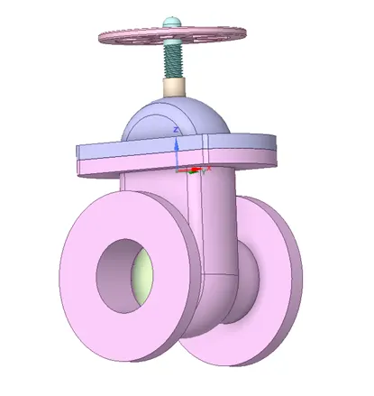
The imported geometry.

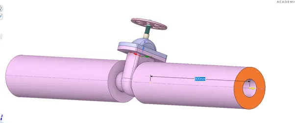
The face has been pulled to extend the volume domain.

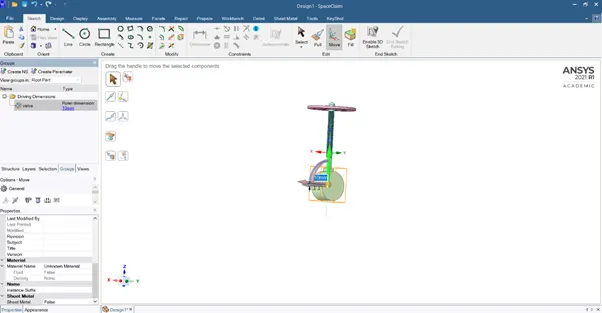
The gate valve disk has been lifted by 10% or 10mm. The value has been set as a parameter. Varying the parameter, the study has been done by increasing it to 80% or 80mm.

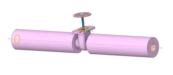
Volume Extracting using SpaceClaim volume-extract function.

 

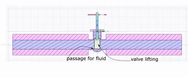
The passage for fluid is the variable section, as the gate valve opens, the passage increases.

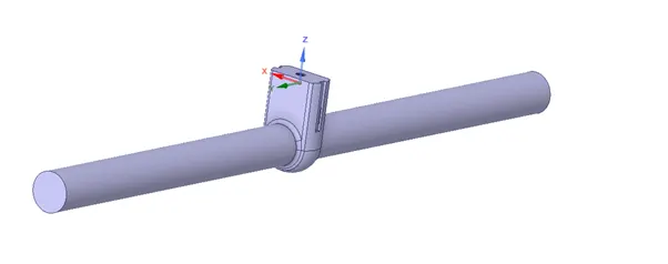
Above is the volume that has been extracted from the given geometry.

MESHING

The defined volumetric domain is then imported to the Ansys meshing module for creating the computational mesh.

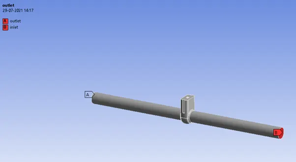
The faces of geometry have been appropriately named to apply boundary condition in the fluent module. The named selection has been shown below.

The element size of the domain is of 0.01m using tetrahedral of 4 faces.

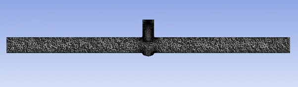
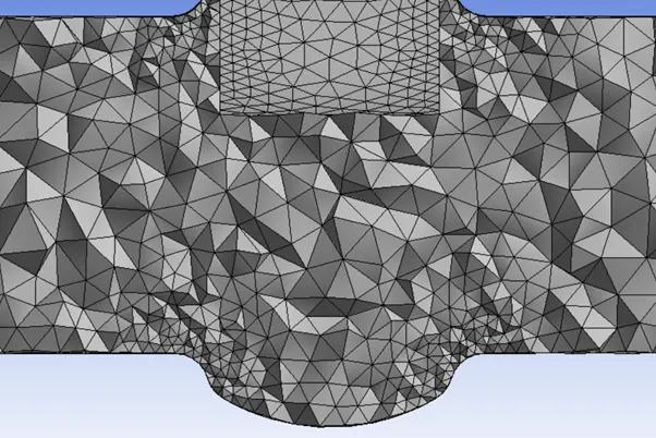
The above picture shows the mesh in the fluid passage area.

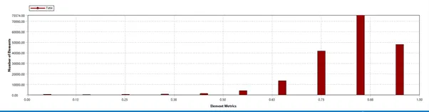
The element quality has been presented below.

SOLVER SETTINGS

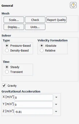
The simulation is run in a steady state, with gravitation enabled to be along the negative of z-axis.

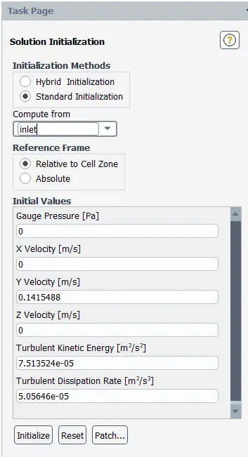
Standard initialization has been used in the present simulation.

Viscous Model

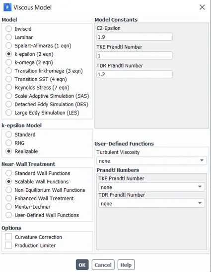
Since this is a pipe flow simulation, if our goal was to employ an accurate solution of near boundary values, we would have gone through modeling the boundary more precisely, here our objective is to measure the bulk flow parameter so we are going to be using K – epsilon model with scalable wall function.

Material Model

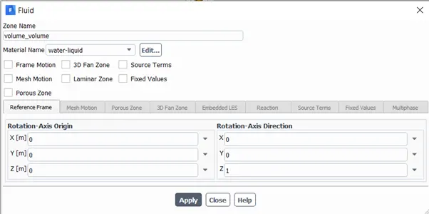
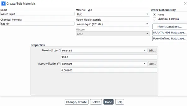
Water is the material of choice for the present simulation. Water material is copied from the fluent database and applied to the volume cell zone.

Boundary Conditions

Inlet

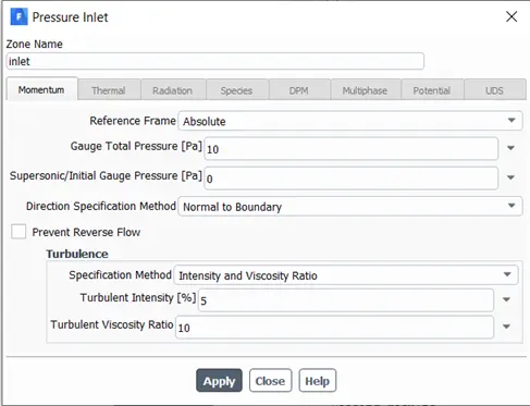
Inlet has been defined as a pressure inlet boundary with a gauge pressure of 10Pa.

Outlet

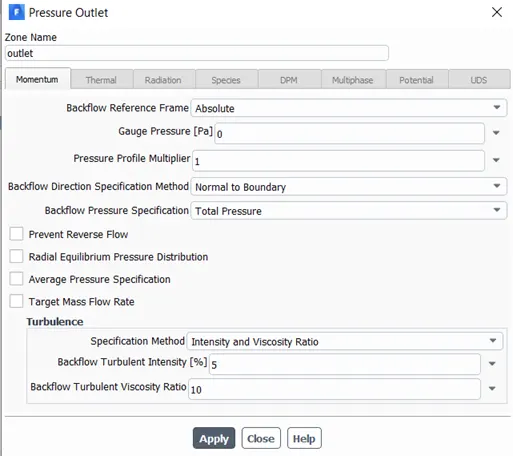
The outlet is a pressure-outlet type of boundary with a value of 0 Pa gauge pressure.

Variables Recording

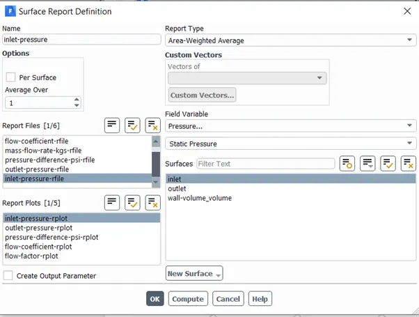
Inlet-pressure (Pa)

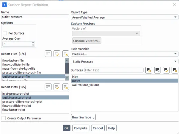
Outlet-pressure (Pa)

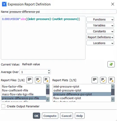
Pressure-difference (psi)

Mass-flow-rate (Kg/s)

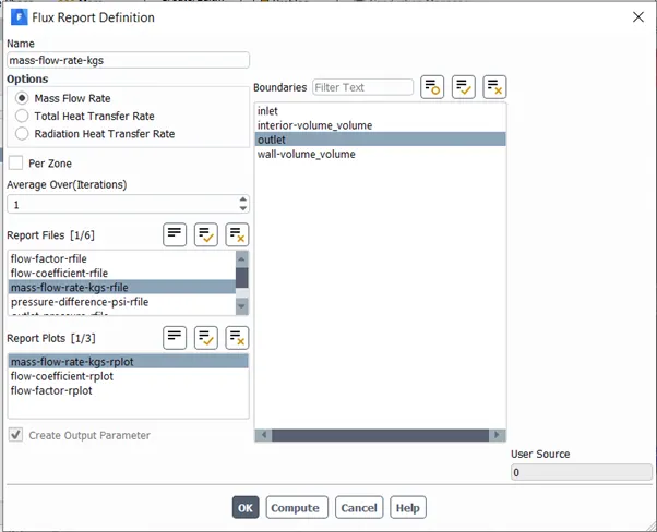
Flow – coefficient

The flow coefficient is calculated using the expression:

Cv=Q⋅SGΔP">Cv=Q⋅√SGΔPCv=Q⋅SGΔP

Where Q is the Volumetric flow rate in Gallons per minute.

ΔP">ΔPΔP is the pressure difference in psi.

The mass flow rate has been converted to Gallon per minute using the multiplication factor (15850.3/998.2) on the mass flow rate(Kg/s)

SG is the specific gravity of fluid flow, in this case, its water, so its value is 1.

 

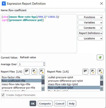
The mass Flow rate and Flow coefficient have been put as output parameters.

Flow Factor is calculated using,

Kv=0.862⋅Cv">Kv=0.862⋅CvKv=0.862⋅Cv

Where,

Kv">KvKv is the flow factor

Cv">CvCv is the flow coefficient

RESULTS:

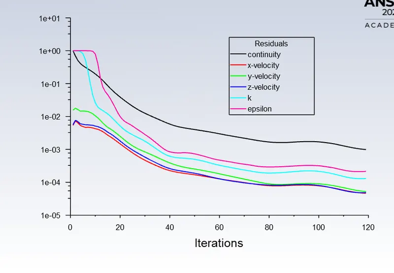
Residual for 10mm gate opening

The Parametric Values gathered from the simulation are:

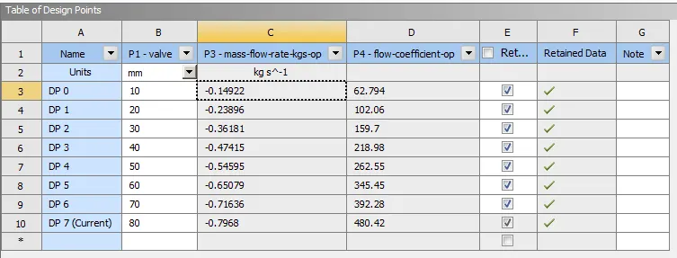
The computed values with flow factor are:

Design Points	Valve Opening [mm]	Mass Flow Rate [Kg/s]	Flow Coefficient	Flow Factor
DP 0	10	-0.14921861	62.793603	54.12808579
DP 1	20	-0.23896146	102.05878	87.97466836
DP 2	30	-0.36180792	159.69514	137.6572107
DP 3	40	-0.47414732	218.97833	188.7593205
DP 4	50	-0.54595204	262.5537	226.3212894
DP 5	60	-0.6507913	345.44977	297.7777017
DP 6	70	-0.7163619	392.27808	338.143705
DP 7	80	-0.79680095	480.41727	414.1196867

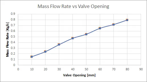
Mass Flow Rate vs Valve Opening

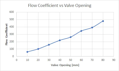
Flow Coefficient Vs Valve Opening

Flow Factor Vs Valve Opening

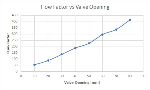
As can be seen from the above plot, The lower the valve, or lesser space is there for fluid flow, low is the mass flow rate.

Also, the lower the valve opening higher the pressure difference. 

With the increase in the valve opening, the mass flow rate also flows coefficient as well as flow factor also increase.