Week 9 - Parametric study on Gate valve.

PARAMETRIC GATE VALVE SIMULATION

Introduction:

Gate valve:

A gate valve is a hydraulic control device used in pipes and conduits to restrict the flow of a fluid. It is also known as sluice valves. The geometry is so simple involving a disc or ball type obstruction fitted inside a bottom and bonnet assembly. The control is usually manual by using a hand wheel. With more advanced electronics being developed, the control can also be automated using IC processors. With fully open condition, there is zero obstruction to the fluid flow. As the pressure increases, friction losses can be a hindrance to achieve flow efficiency. Head loss due to these devices is greatly reduced as these devices are mounted linearly to the flow direction.

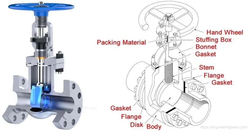
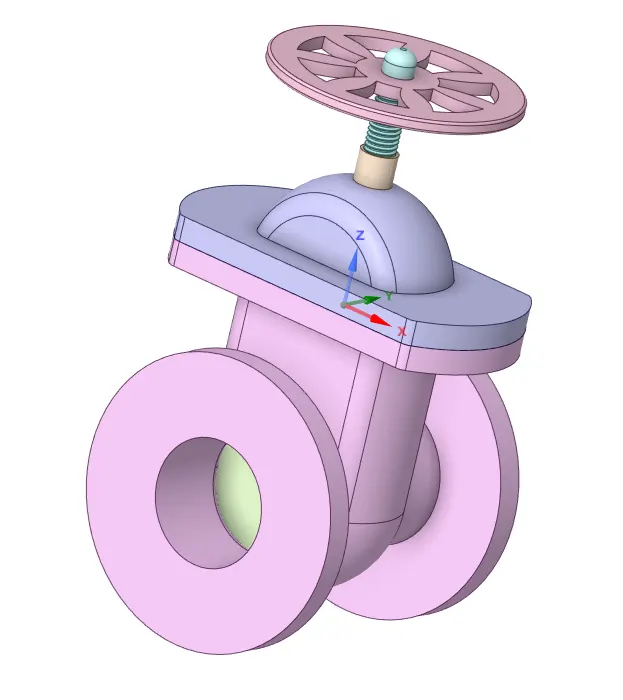
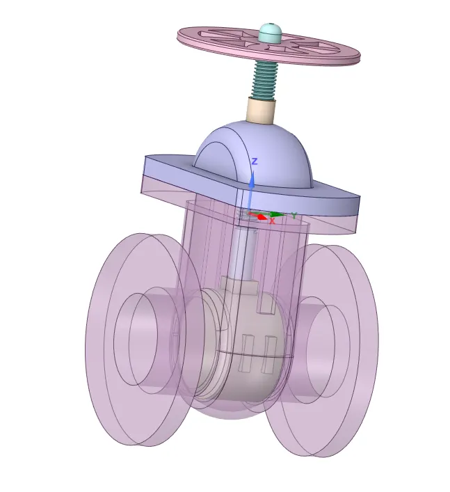
The geometry used here is a disc type manual gate valve with a hand wheel. The pipe diameter is 100mm and for the simulation, the disc is lifted at steps of 10mm each starting from a 10mm lift. The velocity and pressure points are studied along with flow coefficient and flow factor to predict the efficiency of the device.

Flow Coefficient:

The flow coefficient of a device is a relative measure of its efficiency in allowing fluid flow through it. It is the relation between pressure drop across an assembly and the corresponding flow rate.

Flow coefficient, Cv=`Qsqrt((SG)/(DeltaP))`,

where SG is the specific gravity (SG for water is 1) and `Delta P`is the pressure drop in psi and Q is the flow rate in US gallons per minute.

The flow coefficient is useful in comparing valve capacities and sizing valves by way of validating their purpose. The discharge coefficient is used to model the flow equations.

Flow Factor:

It is the metric equivalent factor of the flow coefficient. It is also defined as the water flow in `m^3.h^-1` at a pressure drop across the valve of 1 `(kgf)/(cm^2)`when the valve is completely open. The complete definition also says that the flow medium must have a specific gravity of 1000 `(kg)/(m^3)`and a kinematic viscosity of `10^-6 m^2/s` like water.

Flow factor Kv=0.865.Cv, where kv is in `m^3.h^-1`

Flow factor is derived from the expression, `Qsqrt((SG)/(DeltaP))`

Procedure:

Step 1: Setting up the geometry

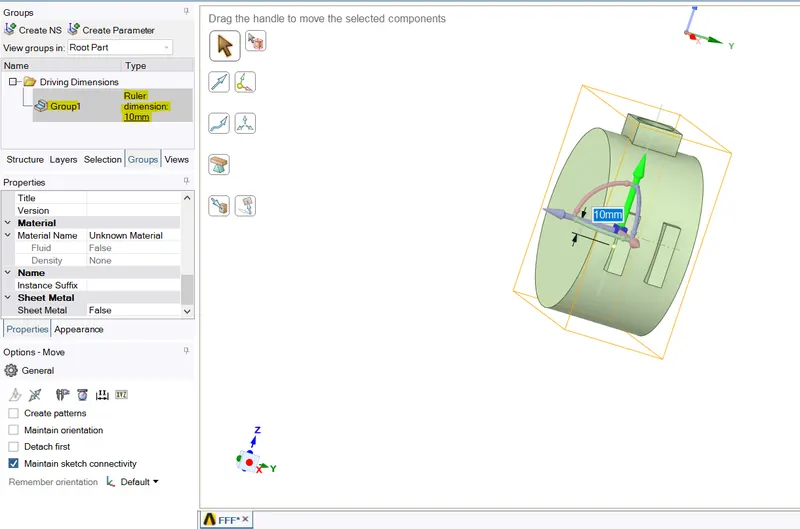
The gate valve disc is parametrized into a group variable. Initially rise of 10mm is given.

The side faces are extended to make fluid volume represent the pipes till 800mm on both sides.

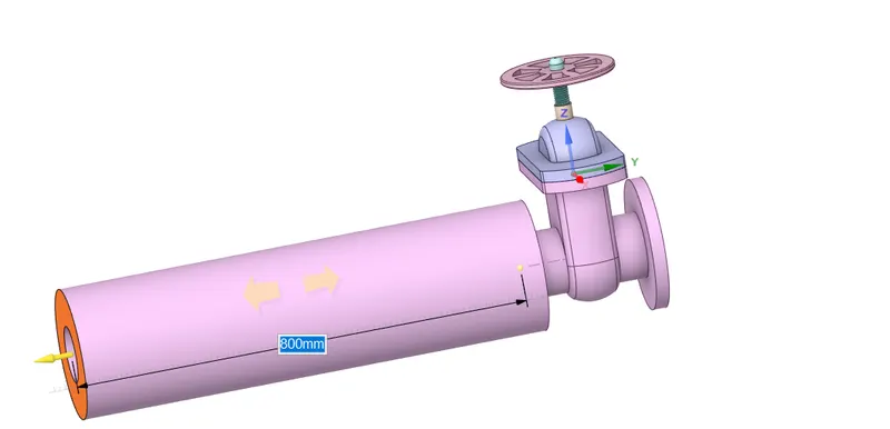
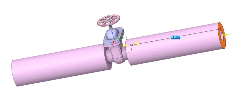
The entire fluid volume is extracted from different edges.

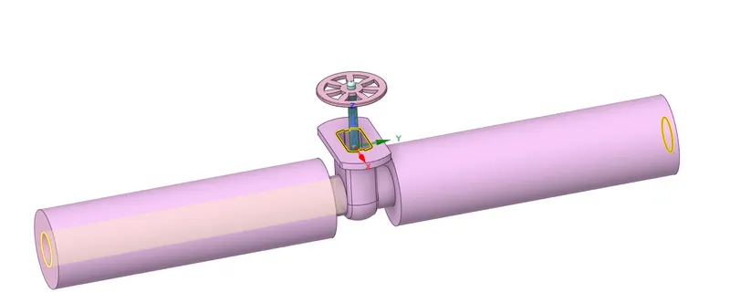
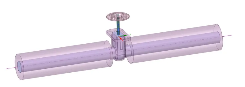
The fluid volume extracted is checked for the corrections in the geometry, and is made to auto align to the valve geometry.

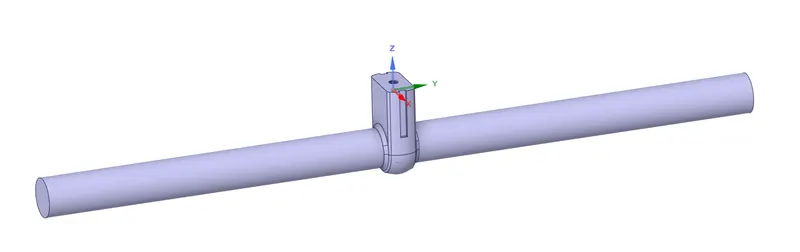
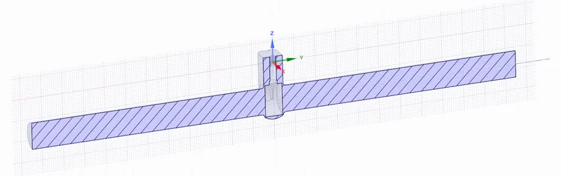
All the geometry except the fluid volume is suppressed for physics.

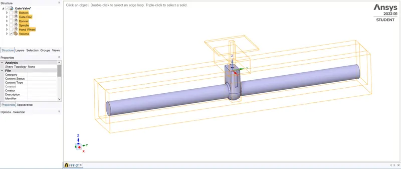
Step 2: Meshing

The inlet and outlet boundaries are named

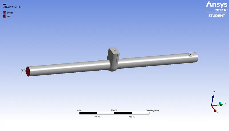
Triangular-faced, tetrahedral cells are taken as default mesh properties, as it is more than convenient for this simulation. The cell size is maintained at 185mm.

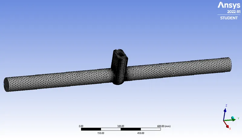
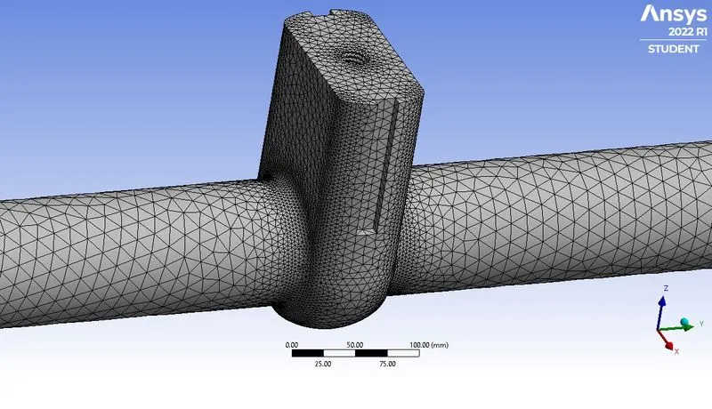
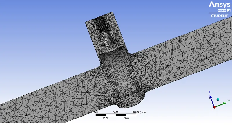
The mesh is generated

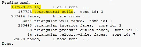
Step 3: Setting up the fluent environment

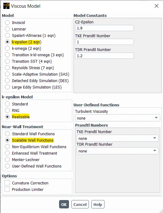
The solver conditions are set to the K-Epsilon turbulence model with a realizable and scalable wall functions method.

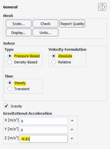
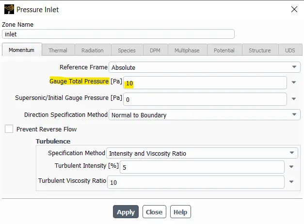
The inlet is set as a pressure inlet and the other boundary conditions are set automatically.

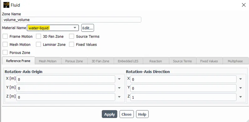
The material is selected as water for the simulation and the air is deleted from the database to avoid miscalculation. The cell zones are updated for the flowing material.

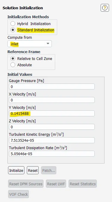
Standard initialization is done.

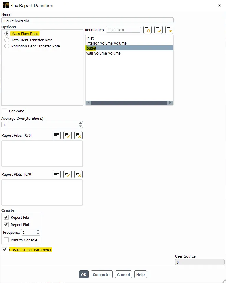
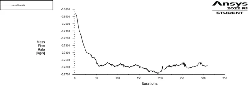
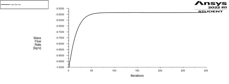
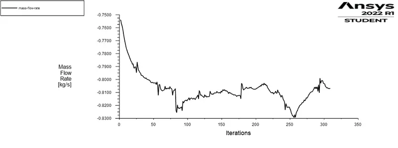
Defining mass flow rate plot computed at outlet is defined.

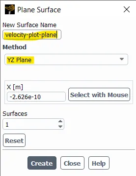
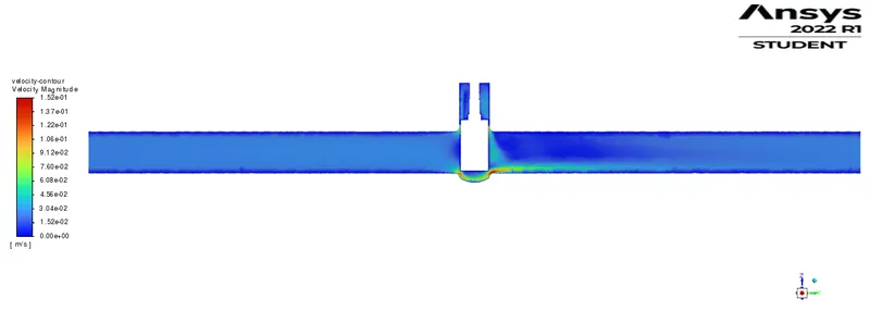
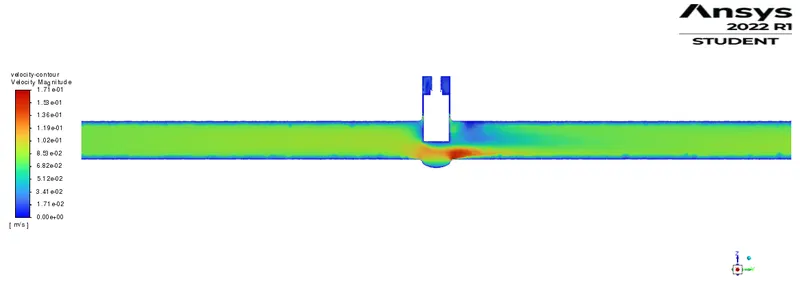
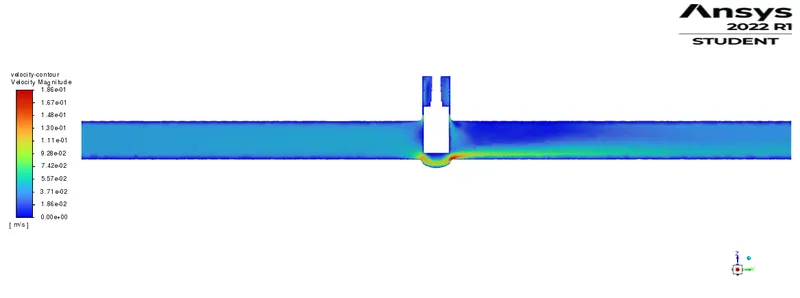
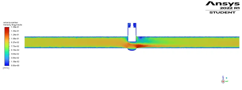
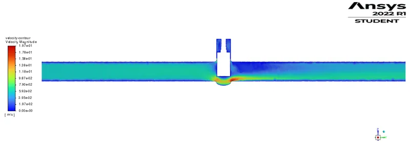
A new YZ plane is defined, and the velocity contour is defined at this plane.

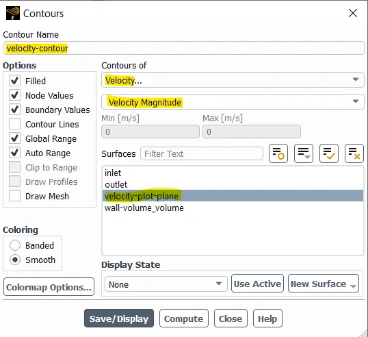
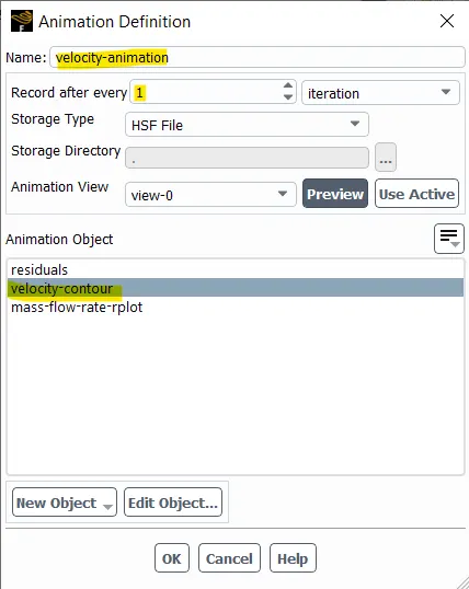
Velocity animation is defined at the velocity contour.

Step 4: Parameter setup

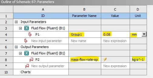
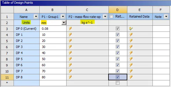
The parameters of disc raise level and mass flow rate level are defined as variables for the simulation. These variables are given at design points.

Run cases:

Case 1	Case 2	Case 3	Case 4	Case 5	Case 6	Case 7	Case 8
Gate valve open condition: 10% (10mm)	Gate valve open condition: 20% (20mm)	Gate valve open condition: 30% (30mm)	Gate valve open condition: 40% (40mm)	Gate valve open condition: 50% (50mm)	Gate valve open condition: 60% (60mm)	Gate valve open condition: 70% (70mm)	Gate valve open condition: 80% (80mm)

Results:

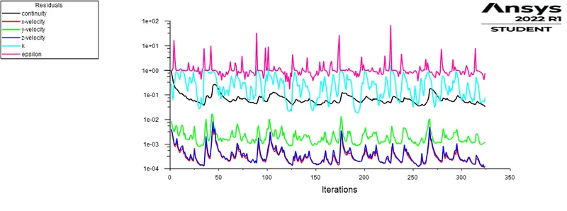
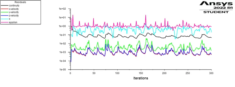
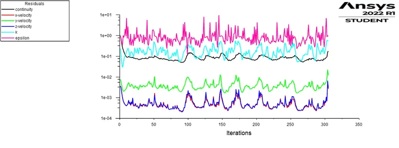
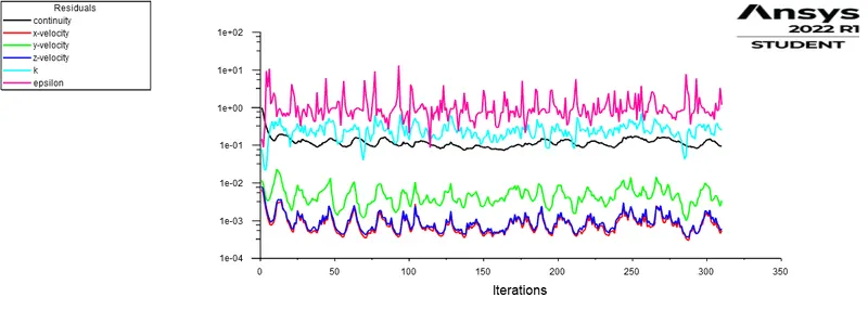
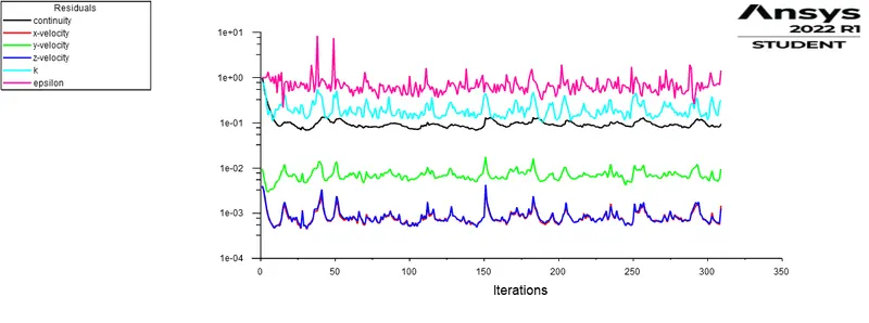
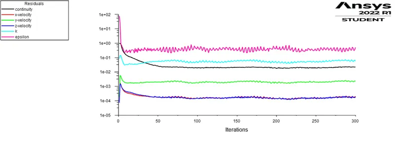
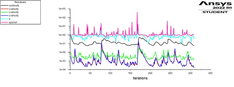
Residuals plot:

Case 1: 10% open	Case 5: 50% open
Case 2: 20% open	Case 6: 60% open
Case 3: 30% open	Case 7: 70% open
Case 4: 40% open	Case 8: 80% open

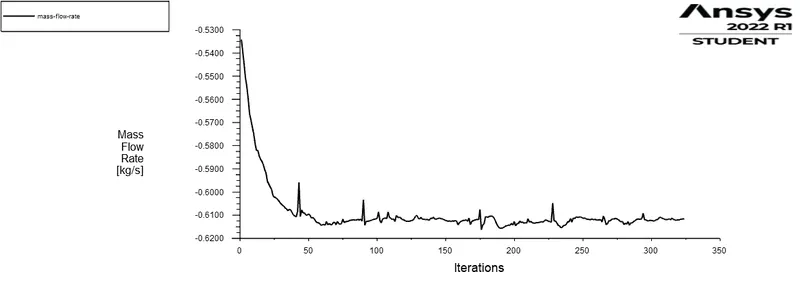
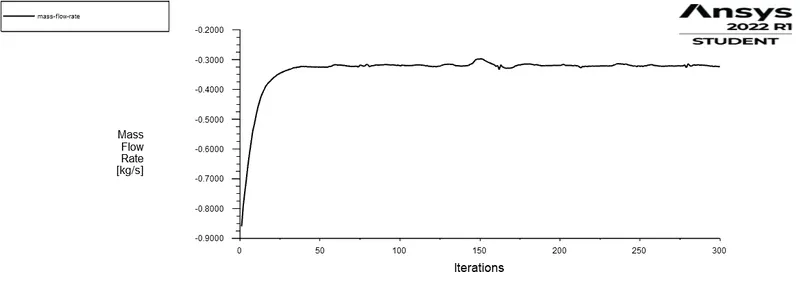
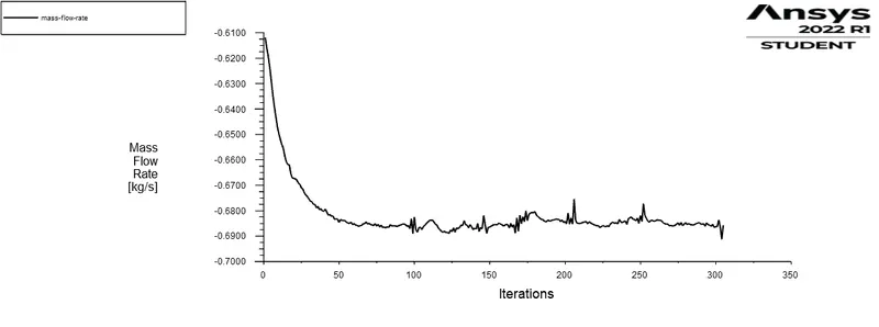
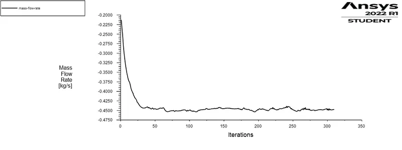
Mass flow rate:

Case 1: 10% open	Case 5: 50% open
Case 2: 20% open	Case 6: 60% open
Case 3: 30% open	Case 7: 70% open
Case 4: 40% open	Case 8: 80% open

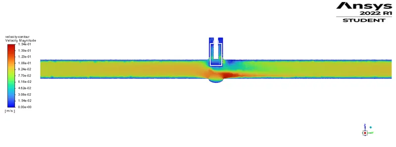
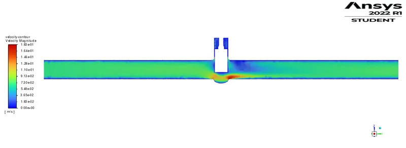
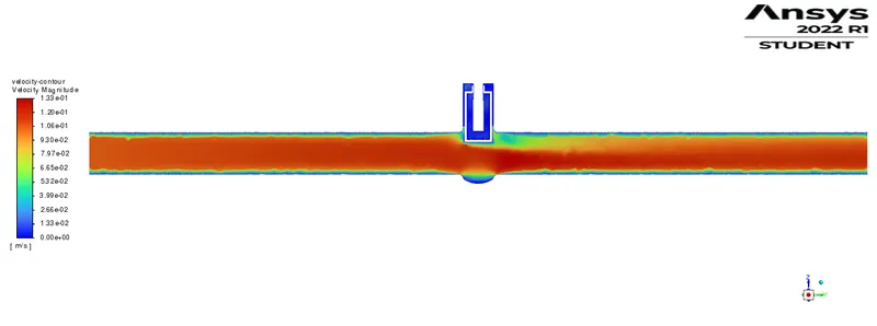
Velocity Contour:

Case 1: 10% open	Case 5: 50% open
Case 2: 20% open	Case 6: 60% open
Case 3: 30% open	Case 7: 70% open
Case 4: 40% open	Case 8: 80% open

Computed values:

	Case 1: 10%	Case 2: 20%	Case 3: 30%	Case 4: 40%	Case 5: 50%	Case 6: 60%	Case 7: 70%	Case 8: 80%
Mass flow rate (kg/s)	0.205	0.322	0.449	0.535	0.614	0.683	0.766	0.808

Conversions: 1kg/s =15.85 US gallons per min

1pascal = 0.000145 psi; 10pascal = 0.00145psi

The specific gravity of water =1

Inference:

	Discharge (US gallons per min)	Flow coefficient (Cv)	Flow factor (Kv `m^-3.h^-1`)
Case 1: 10%	3.249	85.47	73.93
Case 2: 20%	5.103	134.26	116.13
Case 3: 30%	7.116	187.21	161.94
Case 4: 40%	8.479	223.074	192.95
Case 5: 50%	9.731	256.014	221.45
Case 6: 60%	10.825	284.784	246.33
Case 7: 70%	12.141	319.392	276.27
Case 8: 80%	12.806	336.904	291.42

From the above results; it is convenient to observe the flow efficiency of the gate valve under different operating conditions. As the valve disc raises, flow volume increases which increase the efficiency of the device. Hence with an increase in lift, the flow factor and flow coefficient increase.

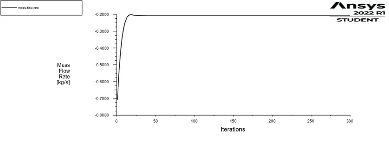
From the velocity contour we can see that, the gate valve provides good control of the velocity of the flow. Comparing the flow between all the cases, the flow efficiency is higher in valves with lift. The mass flow rate also varies accordingly with the necessary lift produces in the valves. Pressure drop is maintained constant across the flow as the velocity is comparatively smaller yet falling in the turbulent flow region. The mass flow rate also increases linearly for the cases which shows that there is linear proportion between the flow values and the output parameters. The durability of the control device can also be predicted using the above given plots. and the flow is seemed to have been achieved steady state.

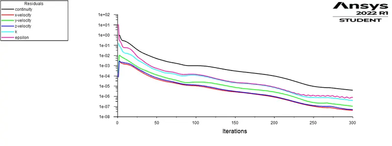
The computed values and the input parameters are clearly in a linear relationship. This conveys that the parameters used and analyzed are fairly convenient for this simulation and the characteristics does not depend on any other parameters other than this. The solution is also seems to be converged after 100 iterations, which proves the efficacy of the solver used.

Case 7	Case 1

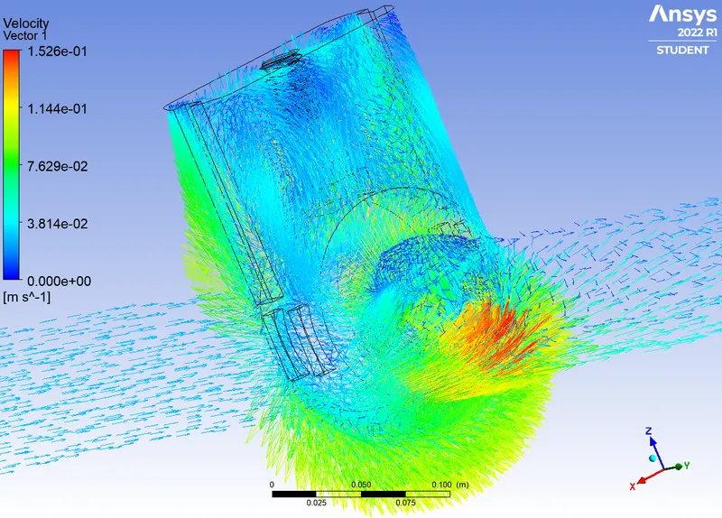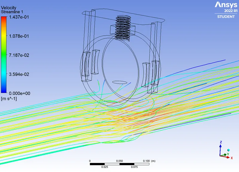
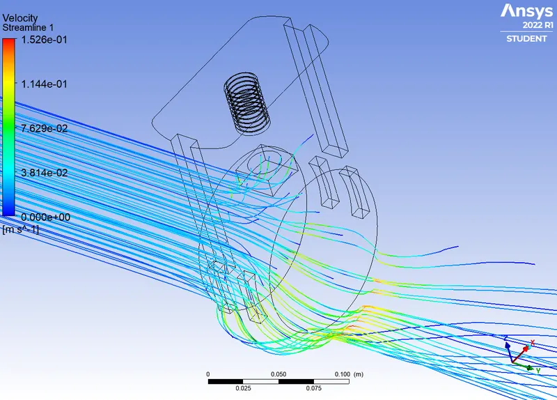
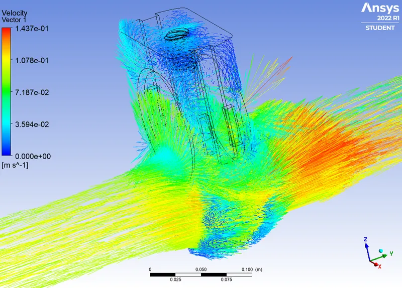
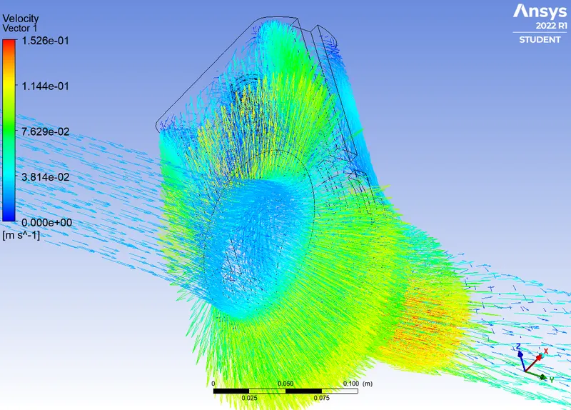
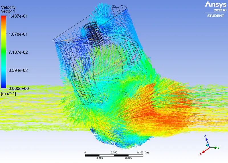
The streamline and vector plots are compared for cases 7 and 1; to identify the critical points and to visualize the flow of the fluid in the 3 dimensional domain. Various points at which the geometry gives resistance to the fluid through friction is also observed. The perfect visualization of working of the gate valve opening and closing is observed in the vector plot.

Conclusion:

Case 1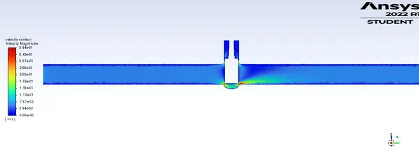
Case 6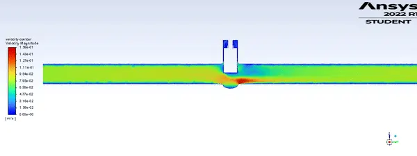

From the above simulation and its result, the working of a gate valve device is studied; and the efficiency of the device, characteristics of the flow are studied by using the parameters being fairly sufficient. Various positions of the gate disc for various flows are studied and the flow characteristics of various flows are visualized using the contour plots.