Week 3.5 - Deriving 4th order approximation of a 2nd order derivative using Taylor Table method

Explanation:

Right side skewed difference scheme:

Order of accuracy (P) = No. of nodes in the stencil (N) – order of the derivative (Q)

N= P+Q

Here: P =2; Q=4 (For 4^th order accuracy of a 2^nd order derivative)

Hence No. of terms = 6

Taylor table:

	f(i)	Δx f’(i)	Δx2 f’’(i)	Δx3 f’’’(i)	Δx4 fiv(i)	Δx5 fv(i)
af(i)	a	0	0	0	0	0
bf(i+1)	b	b	b/2	b/6	b/24	b/120
cf(i+2)	c	2c	4c/2	8c/6	16c/24	32c/120
df(i+3)	d	3d	9d/2	27d/6	81d/24	243d/120
ef(i+4)	e	4e	16e/2	64e/6	256e/24	1024e/120
gf(i+5)	g	5g	25g/2	125g/6	625g/24	3125g/120
Δx2 f’’(i)	0	0	1	0	0	0

Bringing it down to 6 equations and 6 unknowns, using matrix form;

P=

1	1	1	1	1	1
0	1	2	3	4	5
0	½	4/2	9/2	16/2	25/2
0	1/6	8/6	27/6	64/6	125/6
0	1/24	16/24	81/24	256/24	625/24
0	1/120	32/120	243/120	1024/120	3125/120

R= [ a;b;c;d;e;g]

Q= [0;0;1;0;0;0]

Solving by matrix inversion method, R=P^-1 *Q

d²u/dx² = (af(i) +b(f(i+1))+c(f(i+2))+d(f(i+3))+e(f(i+4)+g(f(i+5))) / Δx²

^{Left side skewed difference scheme:}

Order of accuracy (P) = No. of nodes in the stencil (N) – order of the derivative (Q)

N= P+Q

Here: P =2; Q=4 (For 4^th order accuracy of a 2^nd order derivative)

Hence No. of terms = 6

Taylor table:

	f(i)	Δx f’(i)	Δx2 f’’(i)	Δx3 f’’’(i)	Δx4 fiv(i)	Δx5 fv(i)
af(i-5)	a	-5a	25a/2	-125a/6	625a/24	-3125a/120
bf(i-4)	b	-4b	16b/2	-64b/6	256b/24	-1024b/120
cf(i-3)	c	-3c	9c/2	-27c/6	81c/24	-243c/120
df(i-2)	d	-2d	4d/2	-8d/6	16d/24	32d/120
ef(i-1)	e	-e	e/2	-e/6	e/24	-e/120
gf(i)	g	0	0	0	0	0
Δx2 f’’(i)	0	0	1	0	0	0

Bringing it down to 6 equations and 6 unknowns, using matrix form;

S=

1	1	1	1	1	1
-5	-4	-3	-2	-1	0
25/2	16/2	9/2	4/2	½	0
-125/6	-64/6	-27/6	-8/6	-1/6	0
625/24	256/24	81/24	16/24	1/24	0
-3125/120	-1024/120	-243/120	-32/120	-1/120	0

U=[ a;b;c;d;e;g]

T=[0;0;1;0;0;0]

Solving by matrix inversion method, U=S^-1 *U

d²u/dx² = (af(i-5) +b(f(i-4))+c(f(i-3))+d(f(i-2))+e(f(i-1)+g(f(i))) / Δx²

^{Central difference scheme:}

Order of accuracy (P) = No. of nodes in the stencil (N) – order of the derivative (Q) +1

N= P+Q-1

Here: P =2; Q=4 (For 4^th order accuracy of a 2^nd order derivative)

Hence No. of terms = 5

Taylor table:

	f(i)	Δx f’(i)	Δx2 f’’(i)	Δx3 f’’’(i)	Δx4 fiv(i)
af(i-2)	a	-2a	4a/2	-8a/6	16a/24
bf(i-1)	b	-b	b/2	-b/6	b/24
cf(i)	c	0	0	0	0
df(i+1)	d	d	d/2	d/6	d/24
ef(i+2)	e	2e	4e/2	8e/6	16e/24
Δx2 f’’(i)	0	0	1	0	0

Bringing it down to 6 equations and 6 unknowns, using matrix form;

M=

1	1	1	1	1
-2	-1	0	1	2
4/2	1/2	0	4/2	½
-8/6	-1/6	0	1/6	8/6
16/24	1/24	0	1/24	16/24
64/240	1/240	0	1/240	64/240

N=[ a;b;c;d;e;g]

O=[0;0;1;0;0;0]

Solving by matrix inversion method, U=S^-1 *U

d²u/dx² = (af(i-5) +b(f(i-4))+c(f(i-3))+d(f(i-2))+e(f(i-1)+g(f(i))) / Δx²

^{MATLAB Program:}

clear all
close all
clc

x=pi/3;
dx=linspace(pi/10,pi/100000,100);
f=@(x)(exp(x)*cos(x));
g=@(x)(-2*exp(x)*sin(x));
d2f=g(x);
func=f(x);

%Right side skewed system
P=[1 1 1 1 1 1;0 1 2 3 4 5;0 1/2 4/2 9/2 16/2 25/2;0 1/6 8/6 27/6 64/6 125/6;0 1/24 16/24 81/24 256/24 625/24;0 1/120 32/120 243/120 1024/120 3125/120];
Q=[0;0;1;0;0;0];
R=P^(-1)*Q;

%central diff system
M=[1 1 1 1 1;-2 -1 0 1 2;4/2 1/2 0 1/2 4/2; -8/6 -1/6 0 1/6 8/6;16/24 1/24 0 1/24 16/24];
N=[0;0;1;0;0];
O=M^(-1)*N;

%Left side skewed system
S=[1 1 1 1 1 1;-5 -4 -3 -2 -1 0;25/2 16/2 9/2 2 1/2 0;-125/6 -64/6 -27/6 -8/6 -1/6 0;625/24 256/24 81/24 16/24 1/24 0;-3125/120 -1024/120 -243/120 -32/120 -1/120 0];
T=[0;0;1;0;0;0];
U=S^(-1)*T;

central_diff=zeros(1,100);
err_central=zeros(1,100);
rightskew_diff=zeros(1,100);
err_right=zeros(1,100);
leftskew_diff=zeros(1,100);
err_left=zeros(1,100);

for i=1:length(dx)
    central_diff(i)=(O(1)*f(x-2*dx(i))+O(2)*f(x-dx(i))+O(3)*f(x)+O(4)*f(x+dx(i))+O(5)*f(x+2*dx(i)))/(dx(i))^2;
    err_central(i)=abs(central_diff(i)-d2f);
    
    rightskew_diff(i)=(R(1)*f(x)+R(2)*f(x+dx(i))+R(3)*f(x+2*dx(i))+R(4)*f(x+3*dx(i))+R(5)*f(x+4*dx(i))+R(6)*f(x+5*dx(i)))/(dx(i))^2;
    err_right(i)=abs(rightskew_diff(i)-d2f);
    
    leftskew_diff(i)=(U(1)*f(x-5*dx(i))+U(2)*f(x-4*dx(i))+U(3)*f(x-3*dx(i))+U(4)*f(x-2*dx(i))+U(5)*f(x-dx(i))+U(6)*f(x))/(dx(i))^2;
    err_left(i)=abs(leftskew_diff(i)-d2f);
    
end
 subplot(2,1,1)
  hold on
 fplot(d2f,'--')
 xlim([-0.05 0.35]);
 figure(1)
 loglog(dx,central_diff,'linewidth',2,'color','r');
 hold on
 loglog(dx,rightskew_diff,'linewidth',2,'color','g');
 loglog(dx,leftskew_diff,'linewidth',2,'color','b');
 legend('Analytical value at x=pi/3','central difference','Right skewed difference','Left skewed difference')
 xlabel('Grid size(dx)');
 ylabel('Value');
 title('Comparing values of derivative calculated by various difference schemes');
 hold off
 
subplot(2,1,2)
 loglog(dx,err_central,'linewidth',2,'color','r');
hold on
xlim([0.002 0.4]);
loglog(dx,err_right,'linewidth',2,'color','b');
loglog(dx,err_left,'linewidth',2,'color','g');
legend('Central differencing','Right skewed diff.','Left skewed diff.')
xlabel('Grid size(dx)');
ylabel('Absolute error');
title('Comparing 4th order approximation error in calculating d2f/dx2');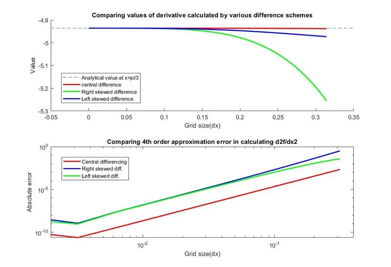

Difference between using different scheme:

From the results, it is inferred that error due to central difference scheme is very small when compared to the other two skewed schemes.

This is because CENTRAL DIFFERENCE SCHEME is simple and is ideal to be implemented on a 2nd order derivative. It does not generate a truncation error term, which is an advantage.

On the contrary side when the grid peclet number goes beyond 2, the scheme may under-shoot or over shoot and becomes unstable.

Thus, the SKEWED DIFFERENCE SCHEMES are necessary to generate a stable solution, when the grid peclet number is more than 2.