Week 9 - Mini project - Flow over an Airfoil
Aim:
- Perform transient state simulation on NACA 2414 Airfoil with varying Angle of Attack
- Calculate the coefficient of Drag and Lift using time-averaged plotdata of Drag force and lift force on the airfoil.
Objective:
- Calculate for the following angle of attacks 1, 5, 10, 15 degrees.
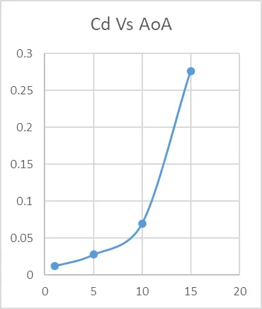
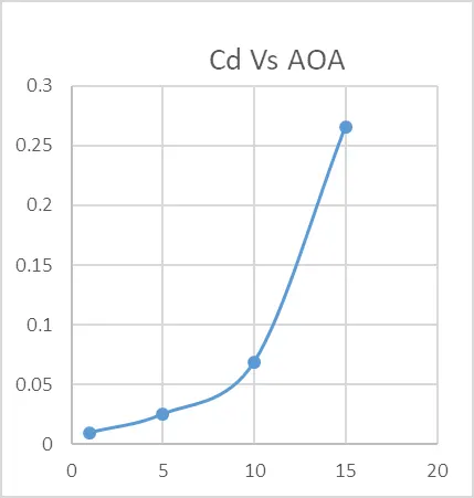
- Drag coefficient Vs Angle of Attack
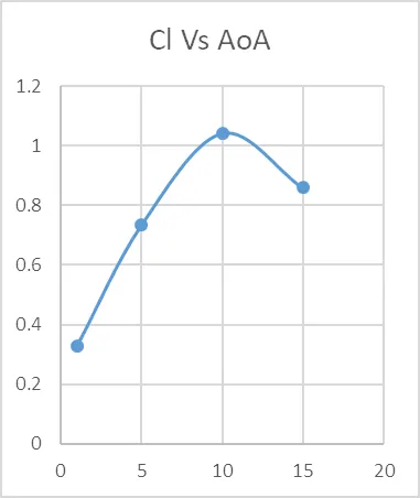
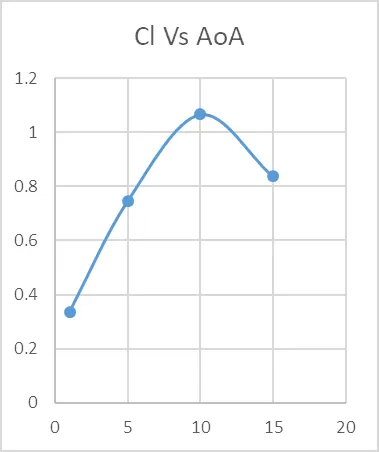
- Lift coefficient vs Angle of Attack
- Compare the effect of turbulence models on the above two results.
Introduction and Theory:
Airfoil, also spelled Aerofoil, shaped surface, such as an airplane wing, tail, or propeller blade, that produces lift and drag when moved through the air. An airfoil produces a lifting force that acts at right angles to the airstream and a dragging force that acts in the same direction as the airstream.
A solid body moving through a fluid produces an aerodynamic force. The component of this force perpendicular to the relative freestream velocity is called lift. The component parallel to the relative freestream velocity is called drag. An airfoil is a streamlined shape that is capable of generating significantly more lift than drag.[1] Airfoils designed for use at different speeds differ in their geometry: those for subsonic flight generally have a rounded leading edge, while those designed for supersonic flight tend to be slimmer with a sharp leading edge. All have a sharp trailing edge.
The lift on an airfoil is primarily the result of its angle of attack. When oriented at a suitable angle, the airfoil deflects the oncoming air (for fixed-wing aircraft, a downward force), resulting in a force on the airfoil in the direction opposite to the deflection. This force is known as aerodynamic force and can be resolved into two components: lift and drag. Most foil shapes require a positive angle of attack to generate lift, but cambered airfoils can generate lift at a zero angle of attack. This "turning" of the air in the vicinity of the airfoil creates curved streamlines, resulting in lower pressure on one side and higher pressure on the other.
Parameters of the Airfoil
Lift and Drag
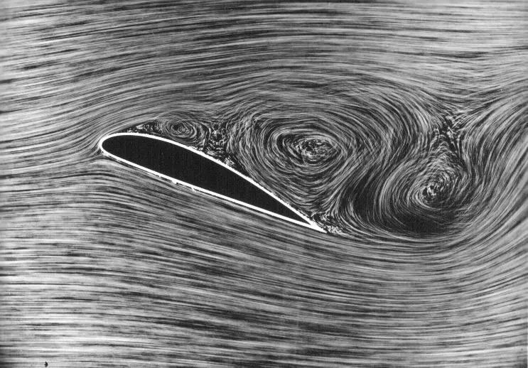
Airflow through the airfoil
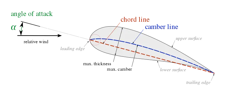
Airfoil terminology:
The various terms related to airfoils are defined below:
- The suction surface (a.k.a. upper surface) is generally associated with higher velocity and lower static pressure.
- The pressure surface (a.k.a. lower surface) has a comparatively higher static pressure than the suction surface. The pressure gradient between these two surfaces contributes to the lift force generated for a given airfoil.
The geometry of the airfoil is described with a variety of terms :
- The leading edge is the point at the front of the airfoil that has maximum curvature (minimum radius).
- The trailing edge is defined similarly as the point of maximum curvature at the rear of the airfoil.
- The chord line is the straight line connecting leading and trailing edges. The chord length, or simply chord,
 is the length of the chord line. That is the reference dimension of the airfoil section.
- The mean camber line or mean line is the locus of points midway between the upper and lower surfaces. Its shape depends on the thickness distribution along the chord;
- The thickness of an airfoil varies along the chord. It may be measured in either of two ways:
- Thickness measured perpendicular to the camber line.
- Thickness measured perpendicular to the chord line.
Some important parameters to describe an airfoil's shape are its camber and its thickness. For example, an airfoil of the NACA 4-digit series such as the NACA 2415 (to be read as 2 – 4 – 15) describes an airfoil with a camber of 0.02 chord located at 0.40 chord, with 0.15 chord of maximum thickness.
The angle of attack:
In fluid dynamics, angle of attack (AOA, α, or {\displaystyle \alpha } ) is the angle between a reference line on a body (often the chord line of an airfoil) and the vector representing the relative motion between the body and the fluid through which it is moving. Angle of attack is the angle between the body's reference line and the oncoming flow. This article focuses on the most common application, the angle of attack of a wing or airfoil moving through air.
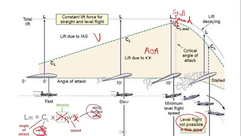
In aerodynamics, the angle of attack specifies the angle between the chord line of the wing of a fixed-wing aircraft and the vector representing the relative motion between the aircraft and the atmosphere. Since a wing can have a twist, a chord line of the whole wing may not be definable, so an alternate reference line is simply defined. Often, the chord line of the root of the wing is chosen as the reference line. Another choice is to use a horizontal line on the fuselage as the reference line (and also as the longitudinal axis).
Relation between the angle of attack and lift coefficient:
The lift coefficient of a fixed-wing aircraft varies with the angle of attack. The increasing angle of attack is associated with increasing lift coefficient up to the maximum lift coefficient, after which lift coefficient decreases.
As the angle of attack of a fixed-wing aircraft increases, separation of the airflow from the upper surface of the wing becomes more pronounced, leading to a reduction in the rate of increase of the lift coefficient. The figure shows a typical curve for a cambered straight wing. Cambered airfoils are curved such that they generate some lift at small negative angles of attack. Asymmetrical wing has zero lift at 0 degrees angle of attack. The lift curve is also influenced by the wing shape, including its airfoil section and wing planform. A swept wing has a lower, flatter curve with a higher critical angle.
Drag:
In fluid dynamics, drag (sometimes called air resistance, a type of friction, or fluid resistance, another type of friction or fluid friction) is a force acting opposite to the relative motion of any object moving with respect to a surrounding fluid. This can exist between two fluid layers (or surfaces) or a fluid and a solid surface. Unlike other resistive forces, such as dry friction, which are nearly independent of velocity, drag force depends on velocity.
Drag force is proportional to the velocity for low-speed flow and the squared velocity for high-speed flow, where the distinction between low and high speed is measured by the Reynolds number. Even though the ultimate cause of a drag is viscous friction, the turbulent drag is independent of viscosity.
Drag depends on the properties of the fluid and on the size, shape, and speed of the object. One way to express this is by means of the drag equation:

where
 is the drag force,
 is the density of the fluid,
 is the speed of the object relative to the fluid,
 is the cross-sectional area, and
 is the drag coefficient – a dimensionless number.
Lift:
A fluid flowing around an object exerts a force on it. Lift is the component of this force that is perpendicular to the oncoming flow direction. It contrasts with the drag force, which is the component of the force parallel to the flow direction. Lift conventionally acts in an upward direction in order to counter the force of gravity, but it can act in any direction at right angles to the flow.
Lift depends on the size of the wing, being approximately proportional to the wing area. It is often convenient to quantify the lift of a given airfoil by its lift coefficient  , which defines its overall lift in terms of a unit area of the wing.
If the value of for a wing at a specified angle of attack is given, then the lift produced for specific flow conditions can be determined:

where,
 is the lift force
- is the air density
- is the velocity or true airspeed
 is the planform (projected) wing area
- is the lift coefficient at the desired angle of attack, Mach number, and Reynolds number
Case Setup:
- NACA 2412 airfoil coordinates were downloaded as ".dat" file and later used to create a closed curve using Solidworks.
- Using the guidelines for bounding box size, the boolean surface was created with airfoil as a tool for subtraction.
- This bounding box or wind tunnel has
width (x-direction) = 50 x Chord Length of the airfoil
Height (Y-direction) = 30 x Chord Length of the airfoil
Distance from the start of the inlet till the leading edge of the airfoil = 25 x Chord Length.
Distance from top of the wall = 15 x Chord Length.
- This Boolean surface was imported in CONVERGE, and later created a copy at an offset of 0.1m in the z-direction.
- Using loft edges, open edges of airfoils and bounding boxes are patched.
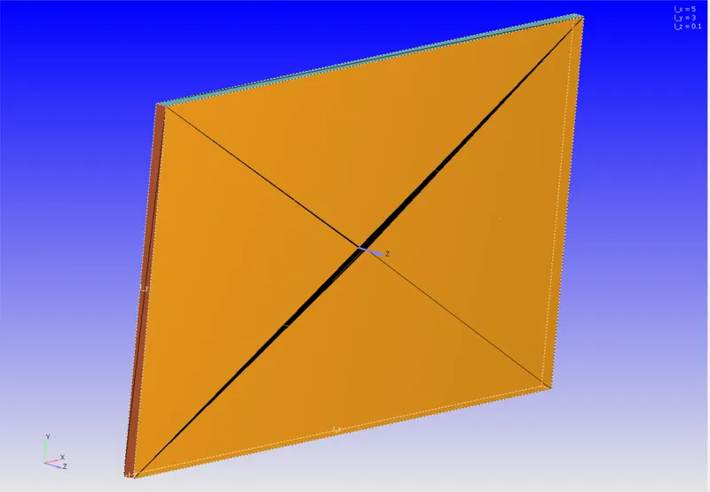
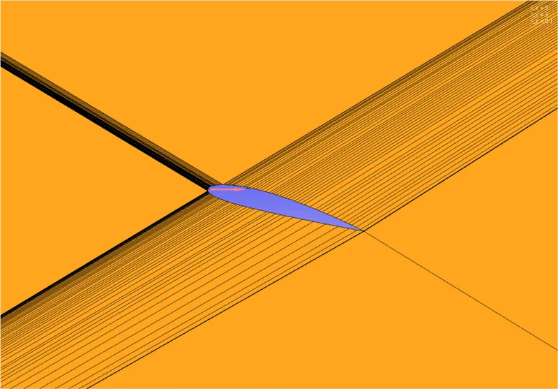
- In Converge Studio, a time-based application is selected and the air is used as a predefined mixture.
- Since this is a transient state simulation case setup, end time was calculated using the flow-through time formula. Flow-through time is the time taken by fluid particles to travel from inlet to outlet boundary with the inlet velocity. In order to estimate this, Inlet velocity was calculated based on the given Reynold's number parameter.
Re = 200000
L = 0.1 m/s
At 300K, following parameters of air are used,
- Using the above-calculated inlet velocity, we can now calculate flow through time,
Flow-through time = Inlet to Outlet total length / Inlet velocity
=
= 0.1593987 sec
rounding off
- As a best practice in transient simulation, the flow has to pass or cycled 3 times through the case. Hence 3x0.16 = 0.48 sec is used as the end time of the simulation.
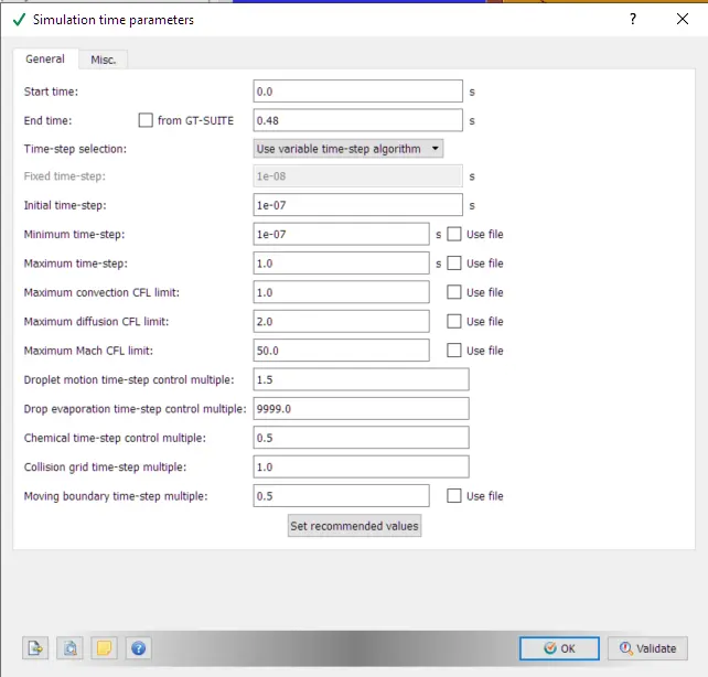
- Region is initialized with the same inlet flow velocity and initial pressure and temperature are at atmospheric.
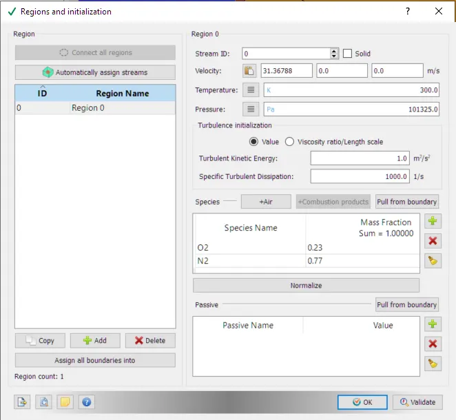
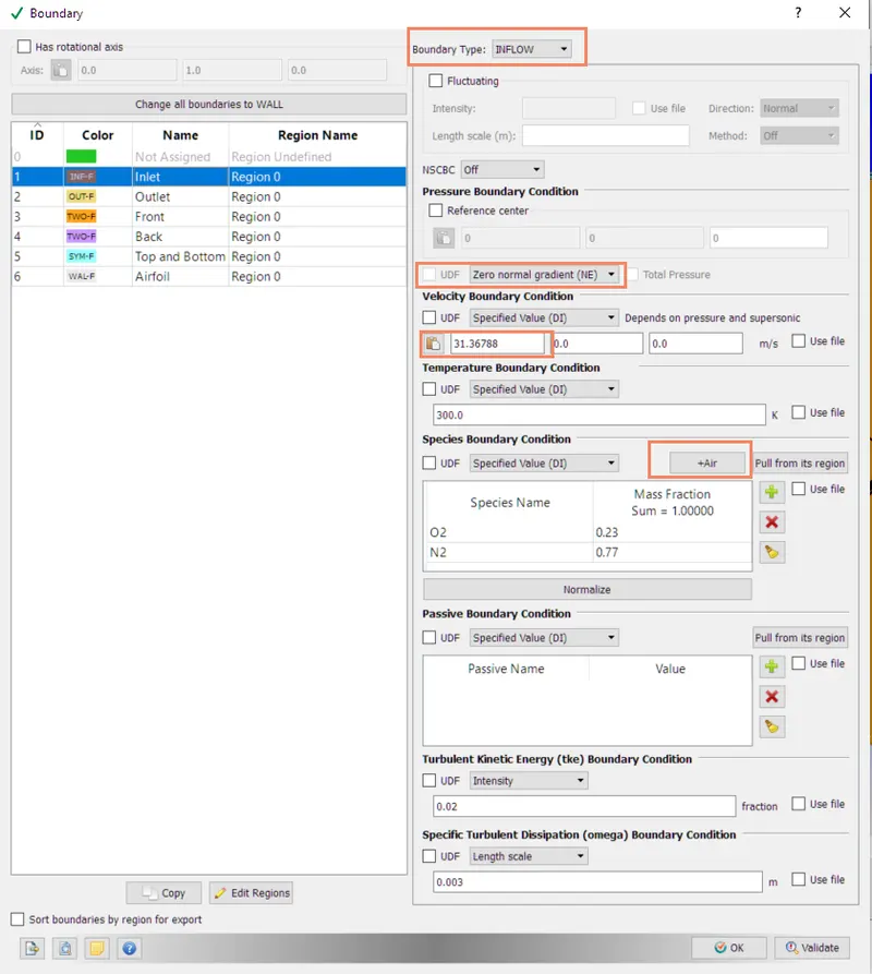
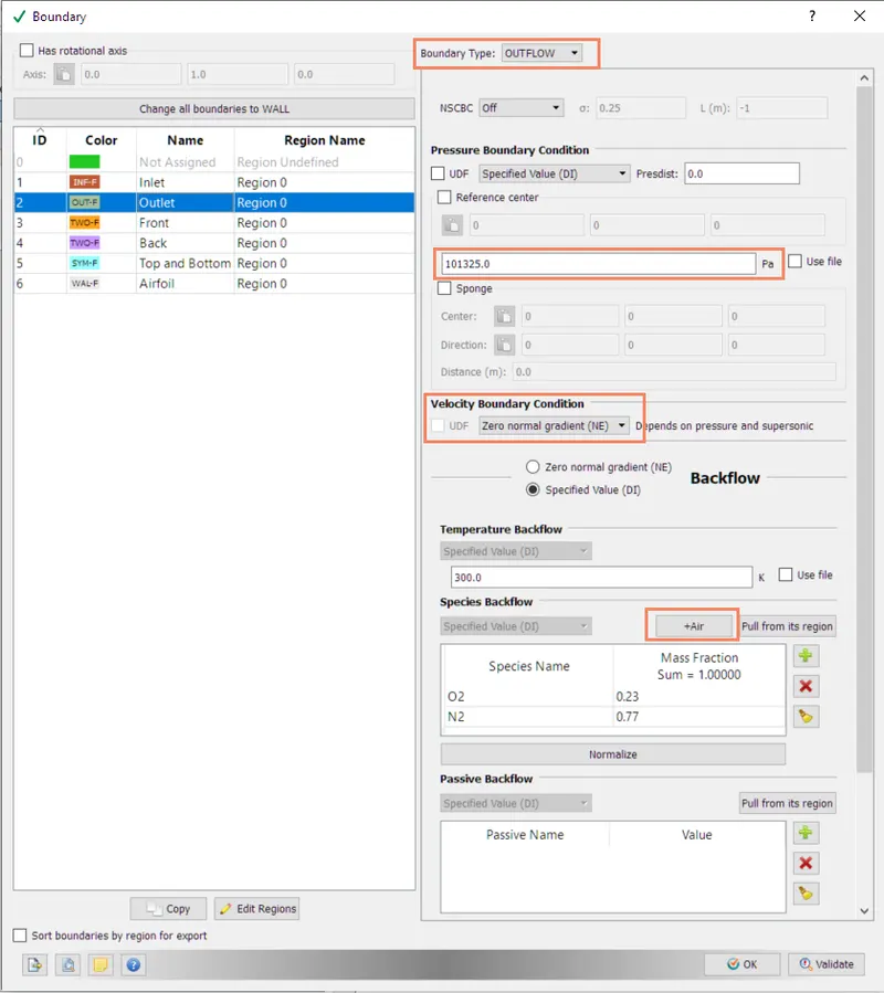
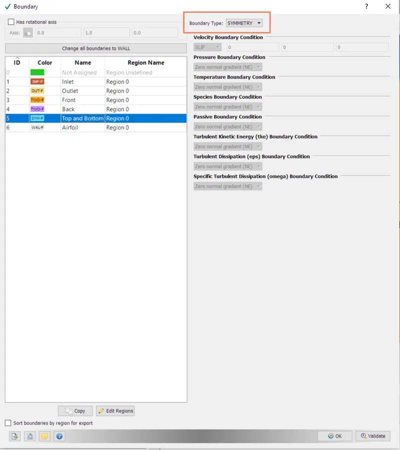
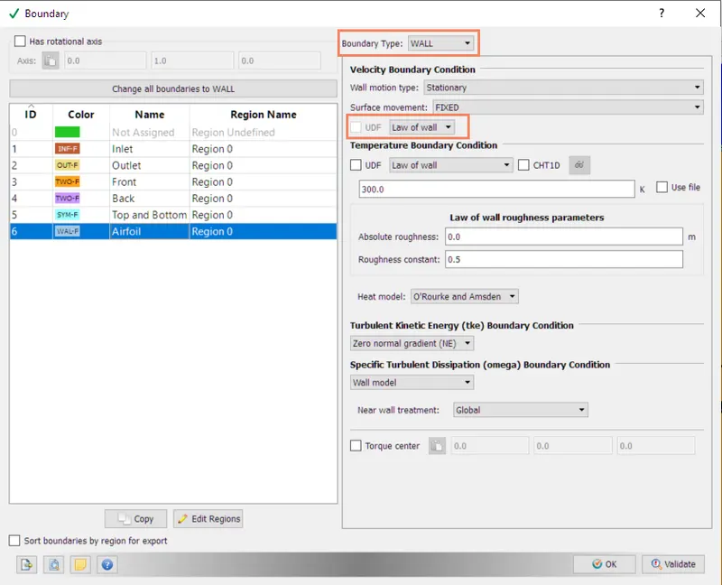
- After that, boundaries have been defined and they have been assigned with following boundary conditions,
- Inlet
- Outlet
- Front and back
- Top and Bottom
- Airfoil surface
- RNG k-
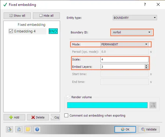
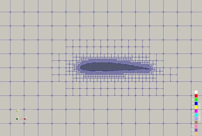
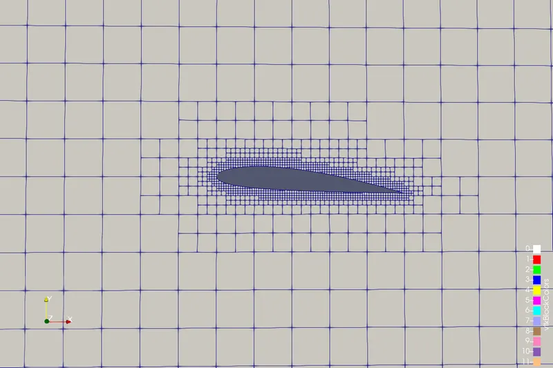
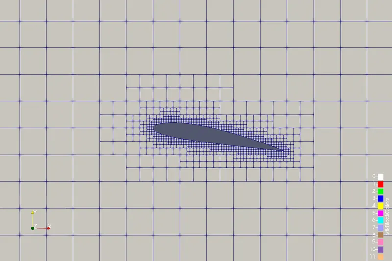
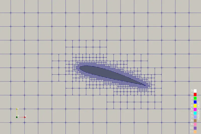
ε ω - Base Grid size of 0.02 m was selected for this test case. In order to have a correct approximation near the wall of the airfoil, fixed embedding is deployed for the entire simulation time. This fixed embedding scale is important to observe the turbulence, flow separation near the wall of the airfoil. Embedding means the refinement of mesh to a lower value than the prevalent base grid size. This is especially useful during the behavior capture of the boundary layer.
- Embedded layers represent the number of refined layers of cells with reduced grid size. The scale represents the decrease in cell size compared to base size. To calculate the scale of fixed embedding, the following formula is used,
First layer thickness = Base Grid Size / 2^n
where n = scale.
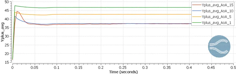
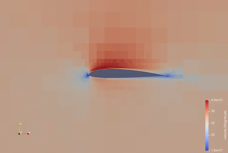
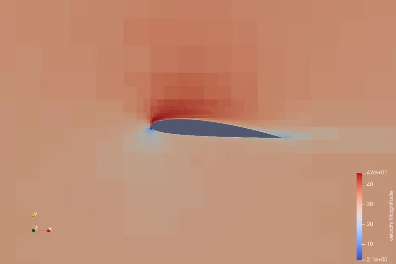
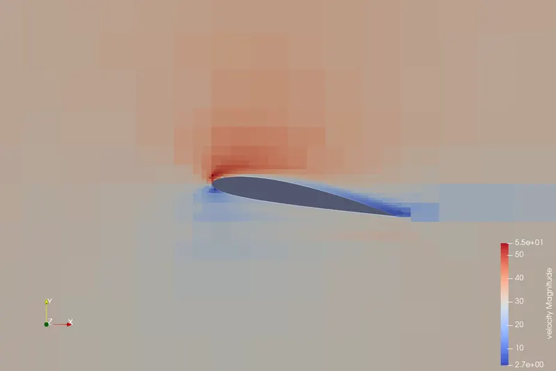
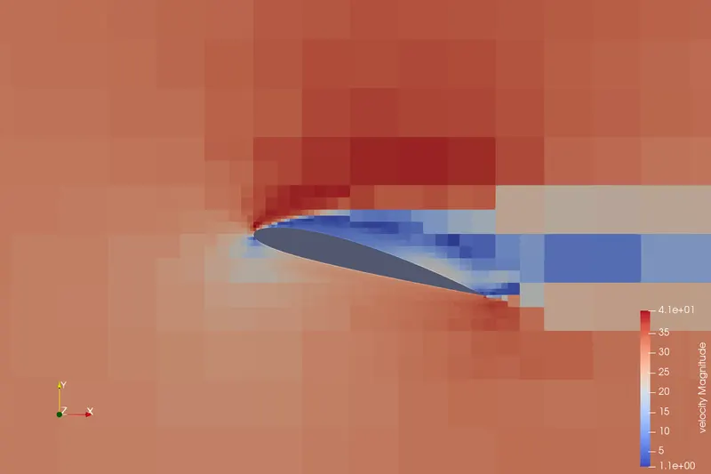
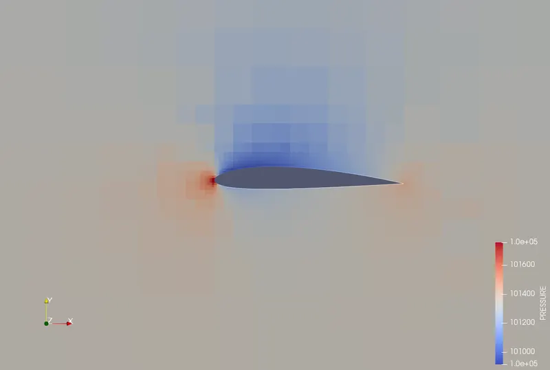
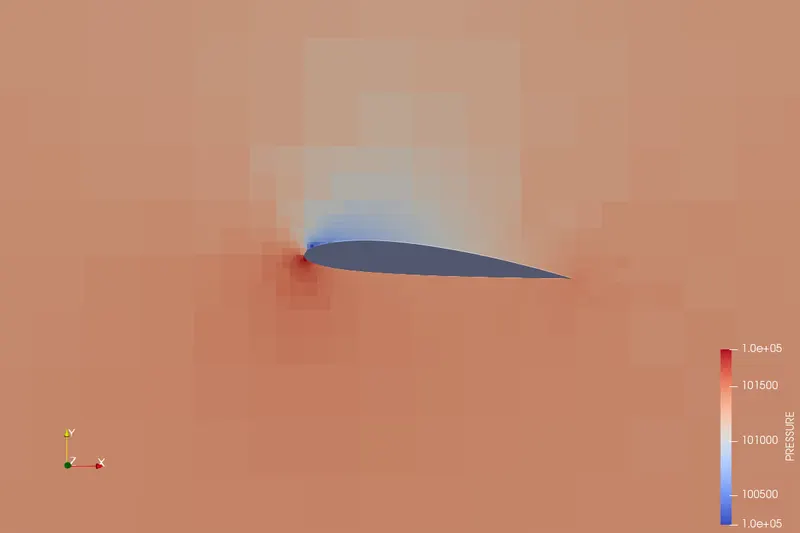
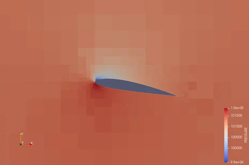
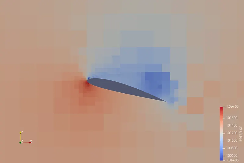
This is interconnected with Y+. First layer thickness is obtained from the Y+ value. For k-epsilon models, the value of Y+ is in the range of 30 to 300. Ideally, the first layer should cover the entire boundary layer and Y+ should be in a turbulent region which is 30 16. After setting up the grid size, variables for post-processing were selected. (velocity, mass flow, pressure, density, temperature) Results: Y+ Average plot Velocity Contour Pressure Contour Considering, A = 0.1 Summary: 1. Transient state solver tends to give better results than steady-state since it uses time averaging method. The contours justify the physics and the plots explain the effect of drag and lift at different angles of attack. 2. Drag increases as the frontal area increases and the lift increases until the flow undergoes flow separation and then the lift reduces and undergoes stall. The dip in the lift force is due to the vortex formation in the leeward side of the aerofoil. 3. in the case of the drag force, the pressure drag component in the total drag is very less in the case of the aerofoil till 10 degrees angle of attack. After the 10degree angle of attack, the pressure drag increases significantly, due to the vortex formation. So the total drag increases. 4. by taking the k - omega SST model, the fluctuations of y+ got reduced. so we can say that we can get accurate results at the walls of the aerofoil using the k-omega SST model compared to the k- epsilon RNG model. 5. the drag and lift force values using both the turbulent models are almost the same. Conclusion: 1. The flow over NACA 2412 at various angles of attacks was simulated. 2. Drag coefficient and lift coefficient were plotted against angles of attack. Also, two turbulence models were used and their effects were studied in this project.
17. After exporting input files, using CYGWIN (command prompt) was used to simulate the project setup.
18. Output files were later converted using CONVERGE studio for post-processing in ParaView.
Angle of Attack
1 Degree
5 Degrees
10 Degrees
15 Degrees
Mesh
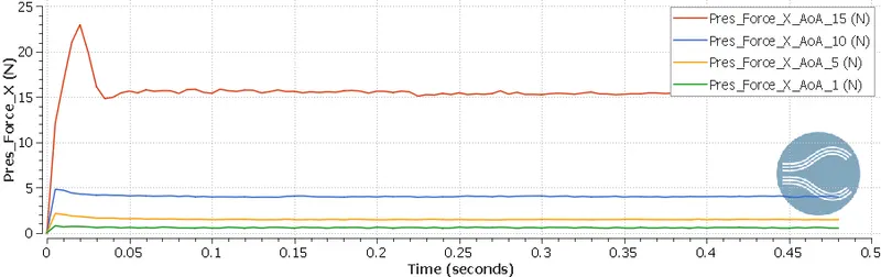
Pressure Force: X
0.56019208 N
1.46228 N
3.992179 N
15.38842 N
Drag Force Plot
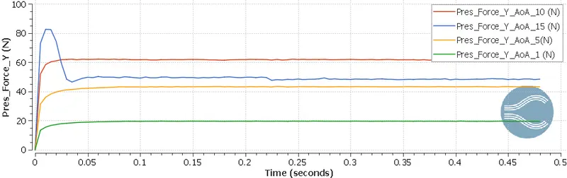
Pressure Force: Y
19.46033 N
43.16703 N
61.75634 N
48.5501 N
Lift Force Plot
RNG k-
Drag Coefficient (
0.009674314
0.025253
0.06894348
0.2657524
Lift Coefficient (
0.336072826
0.7454789
1.06650945
0.8384426
Drag Coefficient (
0.012182
0.027822
0.069622
0.27629
Lift Coefficient (
0.327316
0.733085
1.041212
0.858973