Week - 9 Material Modeling from Raw Data

Processing raw material data to create an LS-Dyna material card

1. Introduction

Material modelling is often one of the challenging steps in any FEA study. The correct representation of the actual case is not possible without providing correct material data in the model. A typical solver contains a number of material cards or templates that are used to describe a material behaviour using an acceptable material model. A generalized practice is to use standard test data (generally referred to as raw data) and convert it to suit the material card available in the solver. A detailed process flow is shown in the figure attached below.

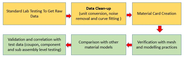
Fig 1.1: The workflow used for material modelling

In this exercise, a true stress-strain curve of graphite iron casting was given and it was asked to model an elastic-plastic material card in LS-Dyna. The created material card needed to be tested using the tensile test of a dogbone model.

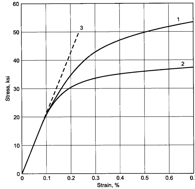
Fig 1.1: The true Stress-Strain data provided for the graphite iron casting

2. Data Extraction

Data points were extracted for curve number 2 in the provided image using a data extraction tool. This data was used for proceeding further with the material modelling process. Generally, a total of 100-200 data points are used for modelling.

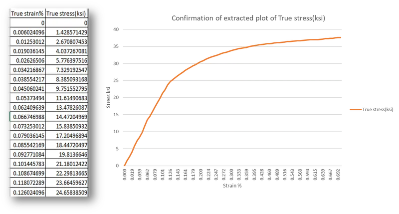
Fig 2.1: The extracted data points and their plot

The plot was used to confirm the accuracy of the data by comparing it with the shape of curve 2 in Fig 1.1. The next step was to clean the data and process it to extract the Young's Modulus of elasticity and Yield point.

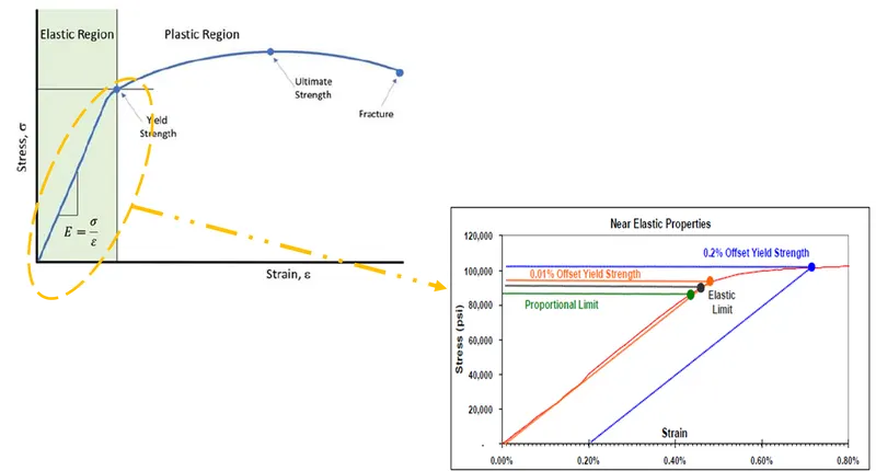
Fig 2.2: The Engineering Stress-Strain curve for a typical ductile material

The general plot of an Engineering Stress-Strain curve obtained using a uniaxial tension test contains the features as shown in the above figure. Some of them are defined as:

• The stress and strain in the first portion of a material’s stress-strain curve are linearly proportional to each other. This forms a straight line on the stress-strain diagram, with a slope known as the Elastic Modulus of the material. The stress level at which the stress-strain response first begins to deviate from linear behaviour is known as the proportional limit.
• The name Yield Strength seems to imply that it is the level of stress at which a material under load ceases to behave elastically and begins to yield. This is not the case. The point at which the material first begins to experience a permanent deformation is known as the elastic limit (shown as the black line in Figure above.) Material that is loaded to a stress level below the elastic limit will completely return to its original size and the shape of the load is released immediately. Conversely, material that is loaded to a stress level greater than the elastic limit will have experienced some degree of permanent deformation.
• The yield strength is defined as the level of stress that produces a specific amount of permanent deformation. This means that by the time the yield strength is reached, the base material has already yielded (undergone permanent deformation) by definition.

Finding the Young's Modulus:

The extracted data was used to find out the elastic modulus using the 'slope' function available in excel. The proportionality limit point in the plot was approximated to 163 MPa stress and data points up to this point were used to find the slope. The result came out to be 142065 MPa which differs by an error of 1.41% from the value (E= 20.9E+6 psi = 144100.5 MPa).

• Some formulae used for conversions are:
• `epsilon_t =ln(1+epsilon)`
• `sigma_t= sigma*e^(epsilon_t)`
• `E.P.S.=epsilon_t-(sigma_t/E)`
• Where `epsilon_t, sigma_t`are true strain and stress, EPS stands for effective plastic strain.

After that, the 0.2% offset yield method was used to locate the yielding point on the curve. This method basically says that a line drawn parallel to the elastic portion of the stress-strain curve passing through 0.2% strain, crosses the stress-strain curve at 0.2% offset yield stress. The overall process is as follows:

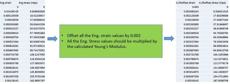
Fig 2.3: The offsetting methodology used

A similar approach was used to offset the values by 0.1% also. All the offset data points were plotted on the engineering Stress-Strain curve as shown in the attached figure.

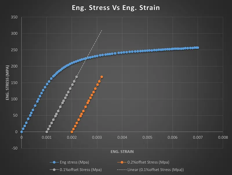
Fig 2.4: The plotting of offset values for finding yield stress

As clear from the above figure, the material seemed to have experienced significant deformation up to the meeting point of 0.2% offset line, so a 0.1% offset line was used instead. This process approximated the Yield stress to be 220.875 MPa.

The next task was to separate the plastic portion of the curve ( after yield point) as only this portion is needed to be keyed into the LS-Dyna material card. A curve fit was found for the plastic portion and this smooth function was used to get evenly spaced 100 data points as shown in the below figure.

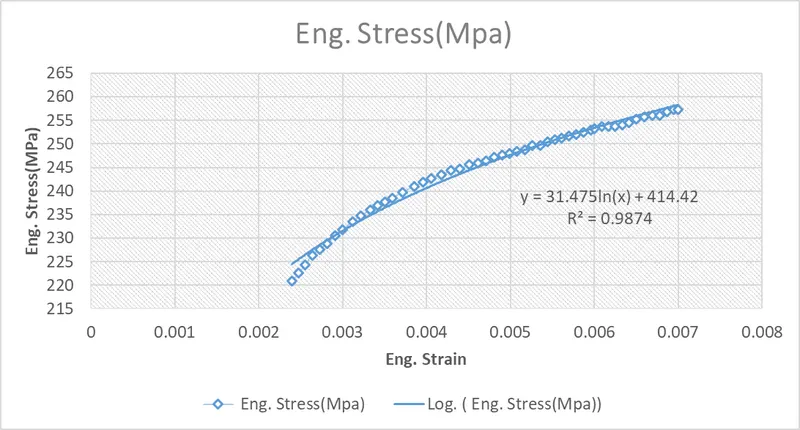
Fig 2.5: The plastic portion of the curve and logarithmic fitted curve

After getting the True stress vs EPS data points these values were fed into Mat 024 piecewise linear plasticity as a stress-strain curve. The unit system used was [kg-mm-ms].

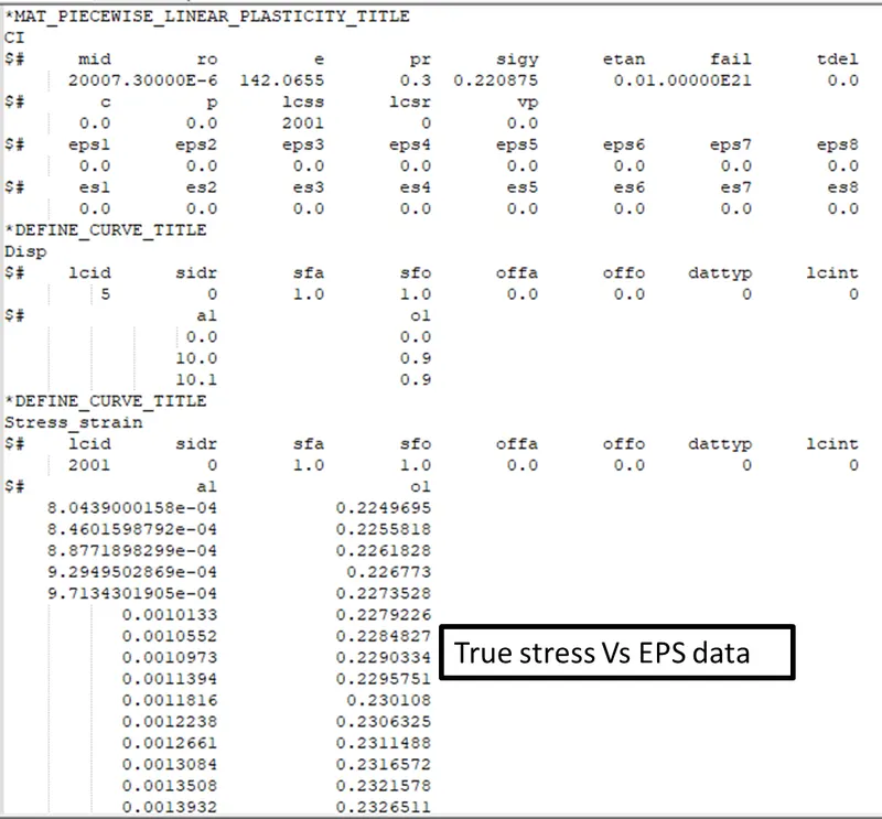
Fig 2.6: The Mat 024 Piecewise linear plasticity card used for the model

3. Tensile test of dogbone model in the LS-Dyna

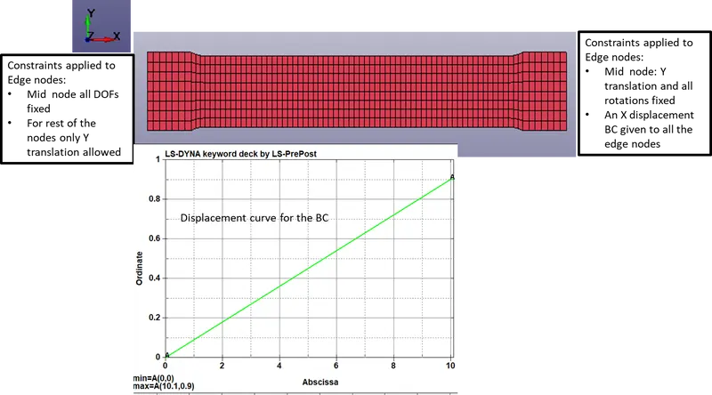
Fig 3.1: the model setup used for tensile test

The strain data provided in the exercise needs the specimen to be loaded up to a maximum strain of 0.7%. This translates to a maximum displacement of 0.9 mm for the 145 mm original length of the specimen.

The implicit simulation was used with a termination time of 5 ms. The implicit solver was used as it is a quasi-static case.

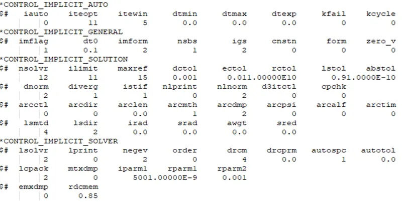
Fig 3.2: The control implicit cards used in the model.

4. Results and discussion

After running the simulation, the stress-strain data for an element in the middle of the specimen was extracted as a CSV file and it was compared with the original true stress-strain data as LSPP gives true stress and strain outputs.

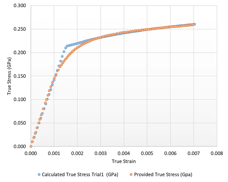
Fig 4.1: The comparison of true stress-strain data calculated by LSPP and the original values

The curve follows well except in the transition region, this miss can be attributed to the errors induced due to curve fitting of the plastic portion and use of inaccurate density and Poisson's ratio.

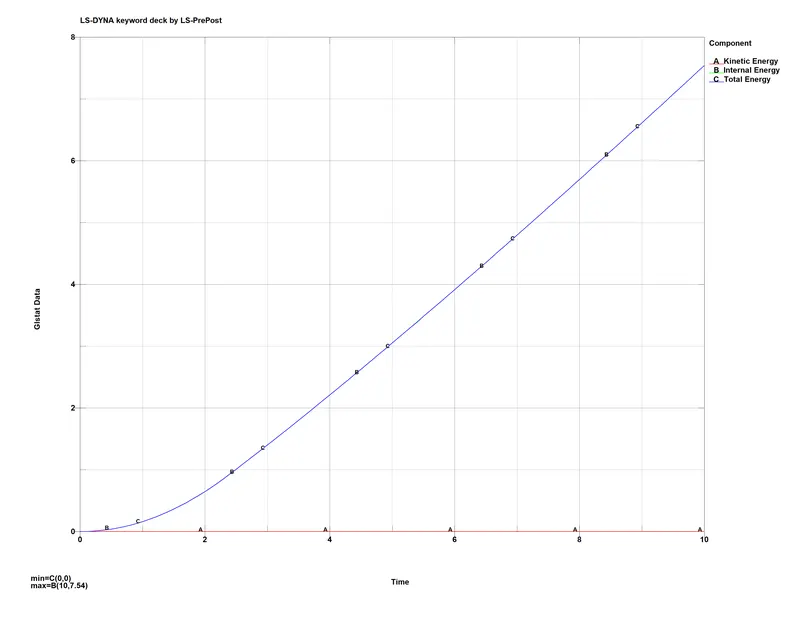
Fig 4.2: The energy plots

AS work was being done on the system its internal and total energy was rising which validates the model to a great extent.

After this, another attempt was made by reducing the Young's Modulus to 180 MPa and again modelling the material. This time the result was better than the previous one.

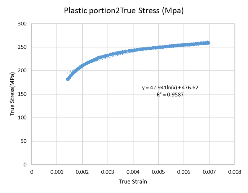
fig 4.3: The 180 MPa stress-strain plot and fitted curve

As clear from the above figure this time the fit was not much accurate, but just as a trial it was used for modelling the material.

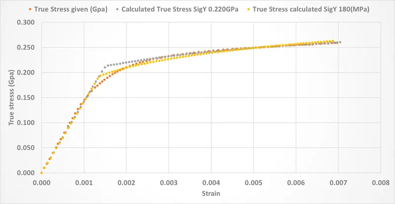
Fig 4.4: The comparison of results using different Young's Modulus values

Conclusion

The 180 MPa yield stress results follow the transition portion more closely but miss the plastic portion due to poor matching of the fitted curve.