Week - 9 Material Modeling from Raw Data

Objective:

By using the diagram of the true stress-strain curve of graphite iron casting. create the material model for the given dog bone specimen. Validate the created material model by performing a tensile test on given specimen, Results are to be compared.

Procedure for material modeling:

• Data extraction from the given curve
• Data clean up and curve fitting
• Data is converted to required unit system
• Defining the stress-strain curve for the material model
• Pre-processing
• Result and Validation

Data extraction from the given curve:

In general material data is collected in the form of:

Foece vs Displacemeny

stress vs strain

Raw data

Image representing the data

Raw data is provided to us, which is representing the true stress and percentage true strain values.

there are three plots with different strain rates. We can see both elastic and plastic region from the curve. Therefore the given data is of a elasto-plastic material.

Here, I have considered the case-2 for the material model.

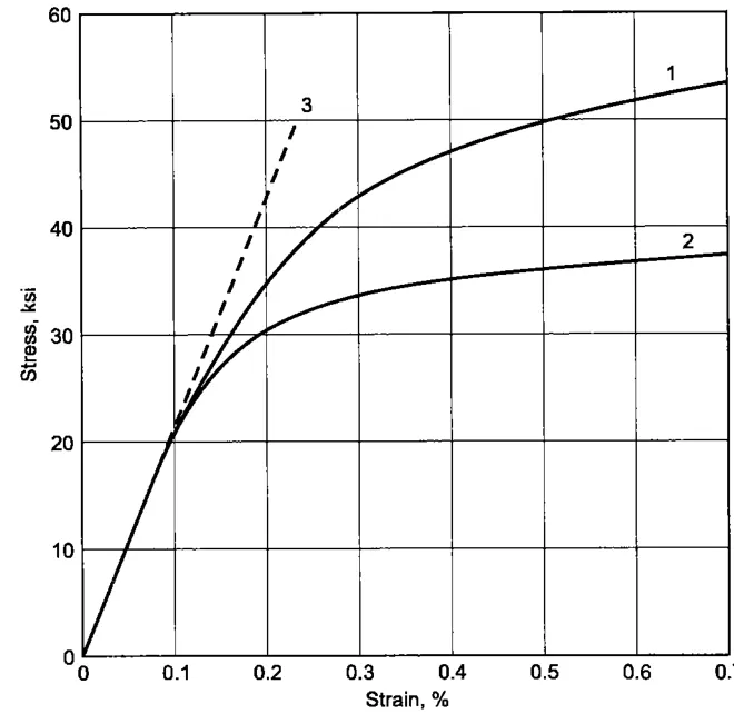
From the given plot, we will take curve data by selecting the data points using GET DATA DIGITILIZER application. The data points are extracted into the excel format.

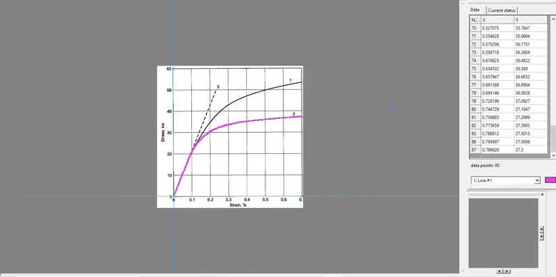
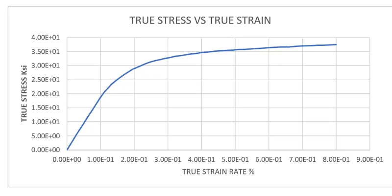
From the data extracted the smooth curve is plotted by removing the kinks and dips causing negative slope.

We can see that the units of stress are in ksi and strain is in Percentage strain.

DATA CLEAN-UP AND CURVE FITTING:

The data is coverted to the required units, i have converted the ksi inti Gpa and Percentage strain into strain.

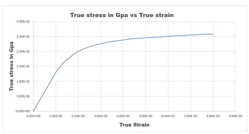
The curve is defined from the values of true stress and true strain obtained from the calculations in excel.

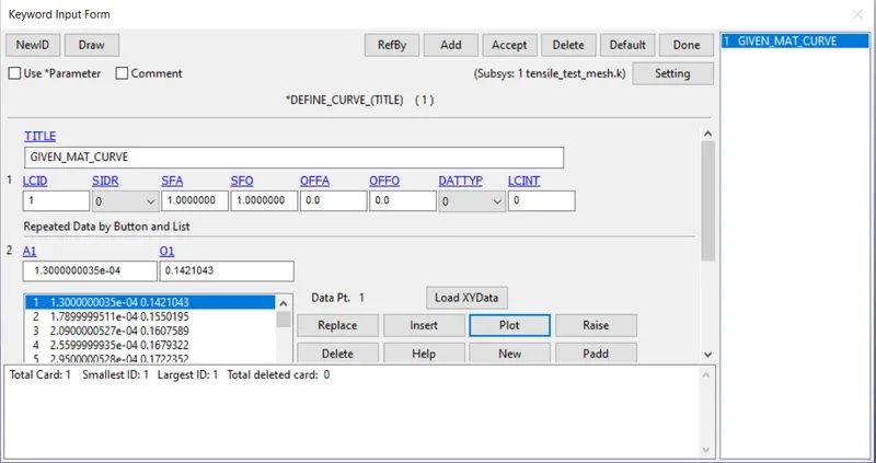
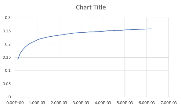
We can see the graph that is the input to the matreial card.

Only plastic region is provided in the material as till the yield, elastic part is calculated with the help of youngs modulus and yield point.

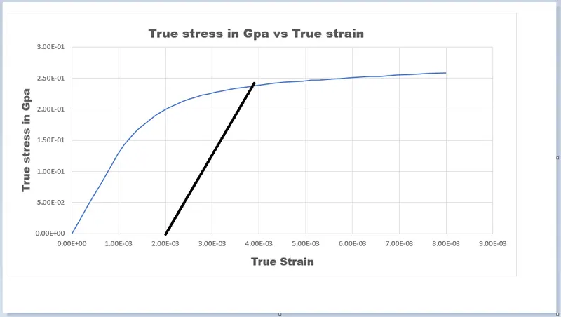
The conversion from elasticity to plasticity can be very subtle for many materials. So, It might not always very easy to figure out the yield point on the stress strain curve, where elasticity changes to plasticity.

In this case Offset yield strength is determined by constructing a parallel line to the Linear curve from 2% strain.

The yield stress obtained = 0.2482 GPa

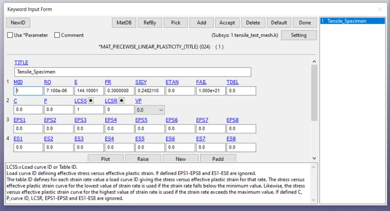
We have to create the material for the specimen. Mat_Piecewise_linear_Plasticity is used in this case.

Density = 7.1 e-06 Kg/mm^3

Youngs modulus = 144.1 GPA

Poissons ratio = 0.3

Sigma y = 0.248211

LSS = 1 ( the above plot is provided )

EPS = Effective Plastic Strain

ES= effective Stress

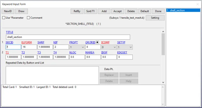
A section has to be created:

ELFORM = 16 is used which is a full integration and thickness is provided to the shell.

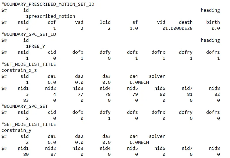
Use appropriate boundary conditions to simulate tensile behavior for the model:

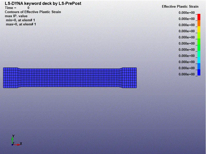
From the below figure we can see that the compression is happening in y-direction and in the other direction, the lateral strain can be seen in the form of bulging out.

Poissons ratio explains this phenomenon, It is defined as the ratio of lateral strain to the longitudinal strain.

We cannot constrain one side of specimen in all degrees of freedom to make it rigid. If we do so, the deformation will be in the tapered manner.

so, we need to constrain in a specific manner as shown below.

1. Constrain all nodes of the side(rigid side) in the x-translation.

2. constrain the set of nodes (middle node on either side of the specimen) in y-direction. These nodes can move in z-direction.

Now, the deformation will take place in a natural way.

Now, we need to provide the prescribed motion on the other side. the degree of freedom is provided in x-direction by constraining all other sides.

We have to provide the displacement i.e calculated from the graph,

which turns out to be, change in length = 1.16435 mm to get the failure data as per the provided plot.

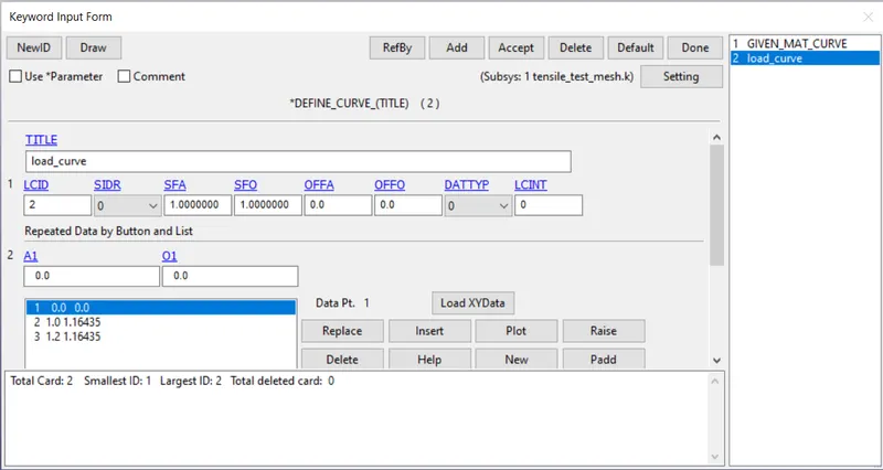
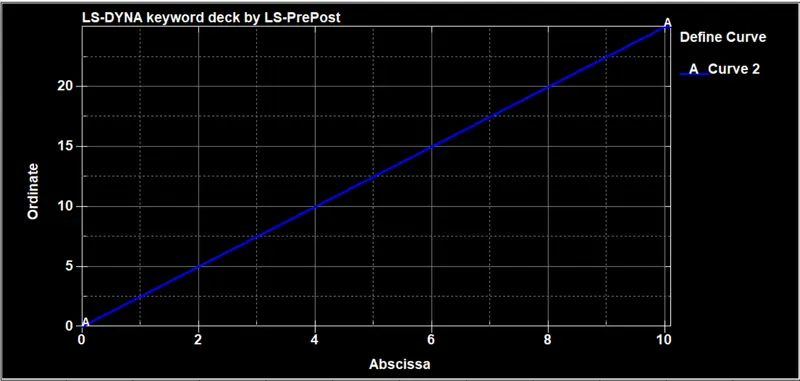
The curve shows how displacement is varying over the time.

We have to define a card to provide the displacement and provide the above curve that is created.

VAD = 2 is representing that the displacement is provided and DOF = 1 is representing the displacement is provided in x-direction.

The node set is created at which the displacement is to be provided and assign it in the*Prescribed_Motion_Set.

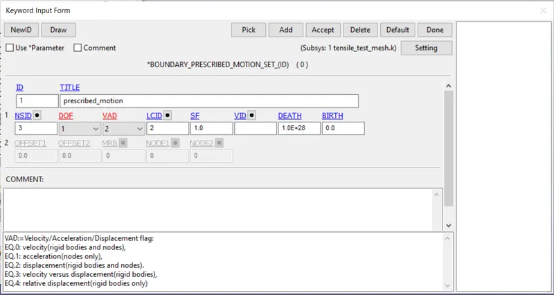
Boundary conditions provided:

Create the control card:

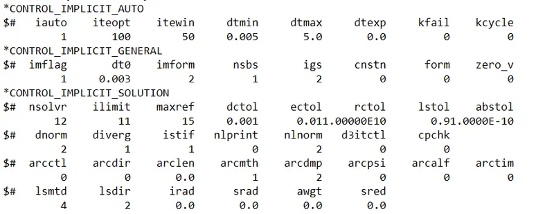
IAUTO = 0 represents the constant time step size.

IAUTO = 1 represents the Automatic adjustion of the time step

ITEOPT is the average number of iterations

ITEWIN is the tolerance value

In this case ITEOPT = 100, ITEWIN = 50

It is representing that, if number of interations is in between 50 (100-50) and 150 (100+50) the time step is going to remain constant.

If less than 50, the time step is increased and if more than 150, the time step is decreased.

In our case, the Automatic adjustion of the time step takes place by using the above data as IAUTO = 1.

IMFLAG = 1 is activating the implicit solver.

Implicit_Solver is represnting the linear solver.

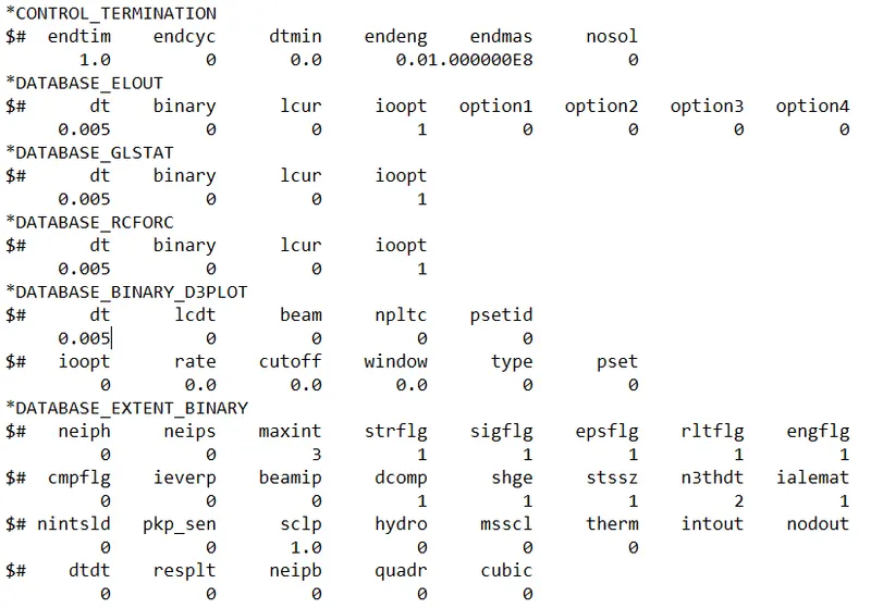
Control_Termination:

The run time of the simulation is given as 1ms.

Create the database card:

Request for D3PLOT:

DT = 0.1 :Time interval at which the animation files should be printed.

*DATABASE_EXTENT_BINARY Flag for output of strain tensors.

Writes strain tensor data to d3plot and elout.
For shell and thick shell elements two tensors are written, one at the innermost and one at the outermost integration point. For solid elements a single strain tensor is written.

Requesting the outputs:

In Database_Ascii >>> Activate GLSTAT, ELOUT, RCFORC

GLSTAT: GLOBAL DATA

ELOUT: ELEMENT DATA

RCFORC: Resultant Internal forces.

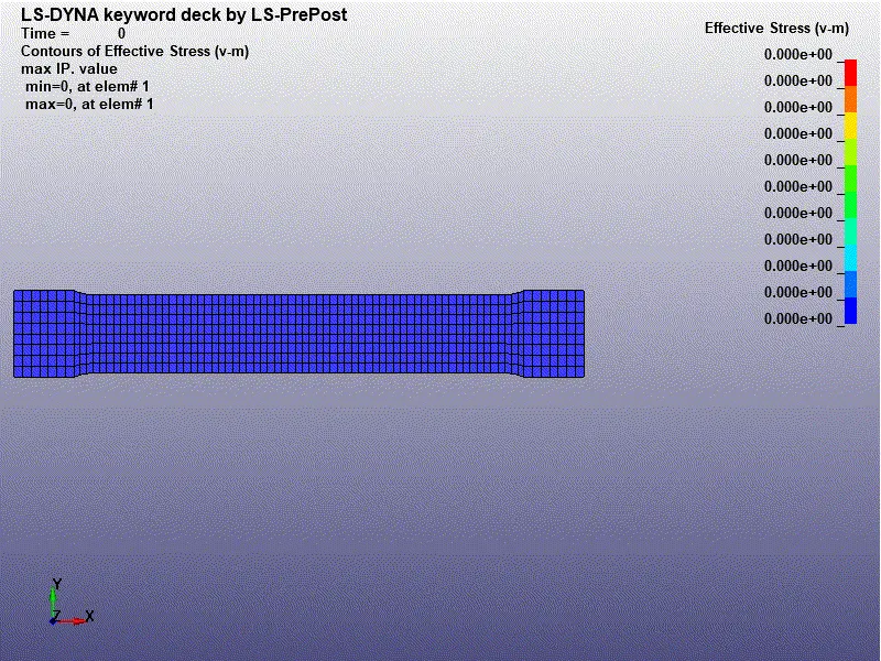
EFFECTIVE STRESS:

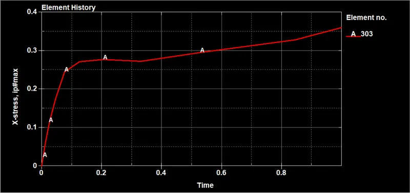
Maximum Stress = 0.27 GPa

EFFECTIVE PLASTIC STRAIN:

Maximum plastic strain = 1.073E-02

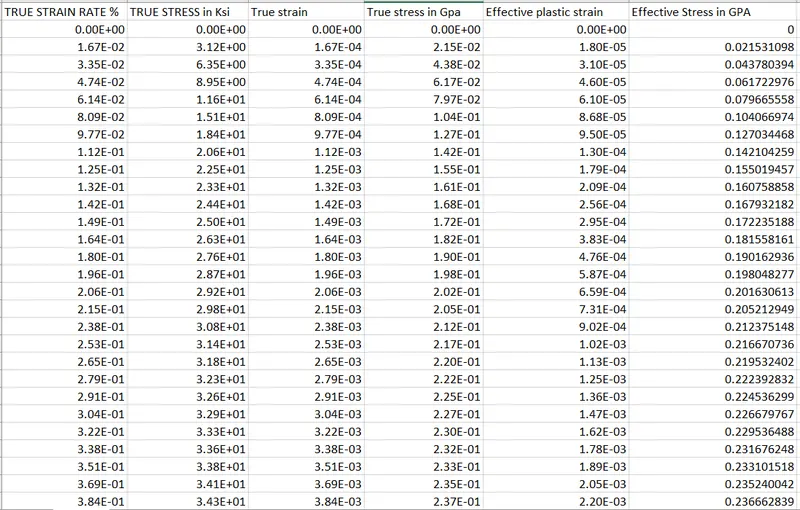
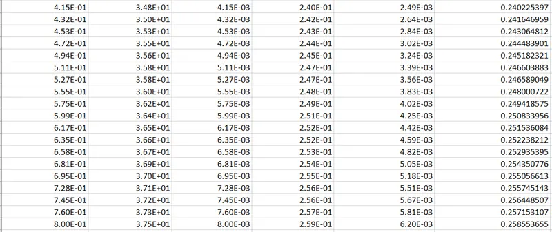
The calculated data is shown below:

Calculation of Effective stress, Effective plastic strain:

ε true = ln (1+ε.eng)

σ true = σ eng (1+ε.eng)

From the true strain rate, true strain is calulatedby dividing true strain rate by 100.

True stress provided is in KSi, i have converted into GPa by using the conversion factor.

Effective plastic strain is nothing but the True stress.

Effective plastic strain is caluculated as shown below

ε effective = ε true - (True stress / Youngs modulus)

The calculated data is shown below.

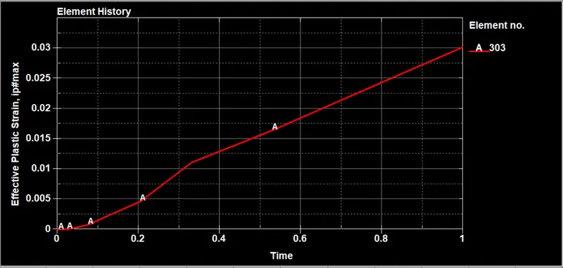
We have selected an element at the cnter of the specimen to see how the stress and strain are taking place:

X-Stress of that particular element with ID 303 is plotted below:

Effective Plastic Strain of that particular element with ID 303 is plotted below:

By cross-plotting the above Effective stress and the effective plastuic strain

Effective Stress vs Effective Plastic Strain of that particular element with ID 303 is plotted below:

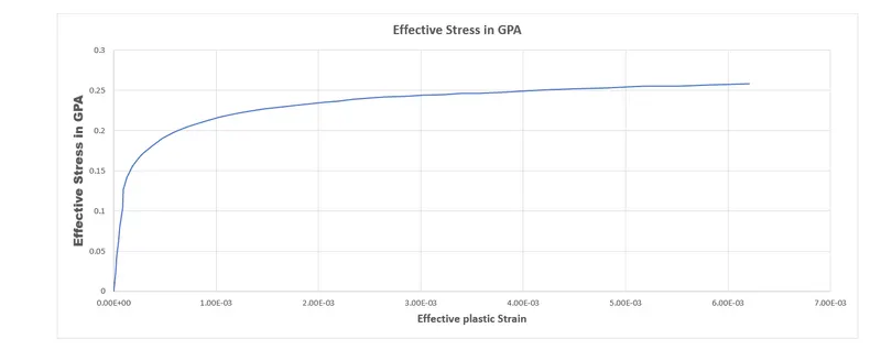
This is the inputted data in the material card:

Only the plastic region data is provided as the elastic region is considered by itself as we have provided the youngs modulus and yield strength.

To see how well our data is matching with the given curve data, Both the Simulated data and the Given data is plotted.

BLUE: Given Data

SAFFRON: Simulated data

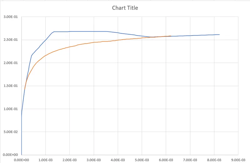
We can see that the graph is converging till the yield point and even at the end of the simulation.

But the convergence is not happenning in between the yield point and end of the simulation.

CONCLUSION:

The stress-strain data extracted from the image is validated with MAT_024 material model.

The stress-strain behavior after the yield point is provided to material card as hardening curve.

The Mat_024 material model captures the actual stress-strain curve in a similar manner and almost matched the defined stress-strain curve. Also, we can see a variation in the simulated data which may be due to not correct density, poissons ratio, mesh size of the model and Improper strain rate w.r.t given data.

This variation can be fine-tuned by trying different values of the above properties and by selecting more data points to capture the give curve better.