Week 9 Challenge: Material Modelling From raw data Challenge

Course: LS-DYNA for Structural Mechanics/ FEA

Submitted by: Amanpreet Singh Whan

Supervisor: Tholkappiyan D

September 01, 2021

Table of Contents

1 Introduction.

2 Aims.

3 Methodology.

4 Results.

5 Conclusion.

1 Introduction

LS-DYNA is an advanced general-purpose multiphysics simulation software package developed by the former Livermore Software Technology Corporation (LSTC), which was acquired by Ansys in 2019. While the package continues to contain more and more possibilities for the calculation of many complex real-world problems, its origins and core competency lie in highly nonlinear transient dynamic finite element analysis (FEA) using explicit time integration. LS-DYNA is used by the automobile, aerospace, construction and civil engineering, military, manufacturing, and bioengineering industries.

Material modeling is a common process in industries. This process involves testing new material or alloy through experiments to extract the behavior of the new material and then modeling this material using the extracted test data to generate a mathematical equation representing the stress-strain behavior of the material and finally validating this approximate equation with the test data which later can be used while performing any type of simulation.

Material modeling is carried out in most of the industries mainly in Research and development sectors because new materials are preferred by the industries to eliminate certain parameters and impart new ones that could be beneficial for the application like improved fatigue, life cycle, thermal and wear-resistant, eliminating manufacturing costs, etc. This newly modeled material can later be used in any type of engineering analysis (Buckling, linear static, thermal) using FEA tools thus preventing testing upon a physical model over and over again until our result reaches fidelity and thus eliminating the high cost and possible error outcomes.

The purpose of the Week 9 challenge is to create a MAT 024 Piecewise Linear Plasticity material card from the given true stress/ strain raw data and use it to perform a uniaxial tension test of the given dog-bone specimen.

2 Aims

1. Extract true stress/ strain data from the given graph using a data digitizer tool.
2. Create a MAT 024 card after cleaning and converting data into required units.
3. Use the material card to perform the uniaxial test of dog bone specimen and validate the post-processing stress-strain results with the given raw data.

3 Methodology

To model a new material whose data either as 'Force vs Displacement' or 'Engineering Stress vs Strain' is collected through the different physical testing processes. This data must be represented in terms of a mathematical equation that replicates the behavior of the material which then can be successfully used for future engineering analysis. In LS-DYNA, this data is modeled using a MAT_024_PIECEWISE_LINEAR_PLASTICITY material card by defining the Load-Curve parameter and where the new data is fed.

The section also describes different stages that were performed to set up simulation file using an engineering tool LS-DYNA for the completion of the Week 9 Challenge task. These stages can be broadly categorized into creating an input deck containing different cards such as contact, control, database, element, hourglass, Boundary condition, keyword, MAT, node, part, section, and title.

Extracting True Stress-Strain Values from the given graph

The True stress-strain data was extracted from the given graph using the Get Data Graph Digitizer application and curve 2 was selected for the challenge purposes. Later, the extracted true stress-strain values of curve 2 were converted into a kg mm ms unit system and are presented in the table1.

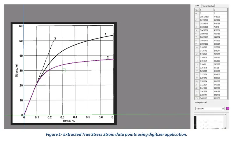
Table 1- Stress Strain Data.

Strain (%)	Stress (KSI)	True Strain	True Stress (GPa)	Effective Plastic Strain
0	0	0	0	0
0.00731627	1.45003	7.31627E-05	0.009997609	3.78325E-06
0.0158561	3.21094	0.000158561	0.022138661	4.92745E-06
0.0256319	5.49033	0.000256319	0.037854508	-6.37632E-06
0.0353828	7.3545	0.000353828	0.050707512	1.93791E-06
0.0439351	9.32301	0.000439351	0.064279916	-6.72621E-06
0.0561456	12.0165	0.000561456	0.082850884	-1.34964E-05
0.0671262	14.2954	0.000671262	0.098563352	-1.27287E-05
0.0805477	17.0922	0.000805477	0.117846617	-1.23319E-05
0.0951865	20.0961	0.000951865	0.138557786	-9.67126E-06
0.109782	22.3733	0.00109782	0.154258534	2.73268E-05
0.120712	23.8217	0.00120712	0.164244904	6.73253E-05
0.132841	25.1658	0.00132841	0.173512151	0.000124304
0.149808	26.8192	0.00149808	0.184911947	0.000214864
0.167974	28.3682	0.00167974	0.195591931	0.000322409
0.18491	29.5025	0.0018491	0.203412657	0.000437497
0.207876	30.738	0.00207876	0.211931133	0.000608042
0.232028	31.6615	0.00232028	0.218298444	0.000805375
0.257378	32.4807	0.00257378	0.223946631	0.001019679
0.281512	33.0928	0.00281512	0.228166914	0.001231732
0.302024	33.6027	0.00302024	0.231682552	0.001412455
0.322531	34.0088	0.00322531	0.234482514	0.001598094
0.341826	34.3116	0.00341826	0.236570247	0.001776556
0.362326	34.6139	0.00362326	0.238654533	0.001967092
0.380417	34.9173	0.00380417	0.240746403	0.002133485
0.402115	35.1152	0.00402115	0.242110876	0.002340996
0.423814	35.3132	0.00423814	0.243476039	0.002548513
0.447922	35.5101	0.00447922	0.244833617	0.002780171
0.467211	35.7091	0.00467211	0.246205674	0.00296354
0.486494	35.8043	0.00486494	0.246862055	0.003151815
0.505783	36.0034	0.00505783	0.248234802	0.003335179
0.529892	36.2002	0.00529892	0.249591691	0.003566852
0.554	36.3971	0.00554	0.250949269	0.003798511
0.575692	36.4913	0.00575692	0.251598756	0.004010924
0.5998	36.6882	0.005998	0.252956334	0.004242583
0.619083	36.7834	0.00619083	0.253612715	0.004430858
0.641981	36.877	0.00641981	0.254258065	0.00465536
0.667294	37.0734	0.00667294	0.255612195	0.004899092
0.685372	37.1691	0.00685372	0.256272024	0.005075293
0.699835	37.2665	0.00699835	0.256943574	0.005215263

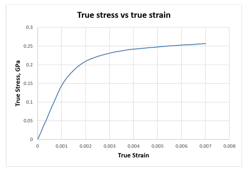
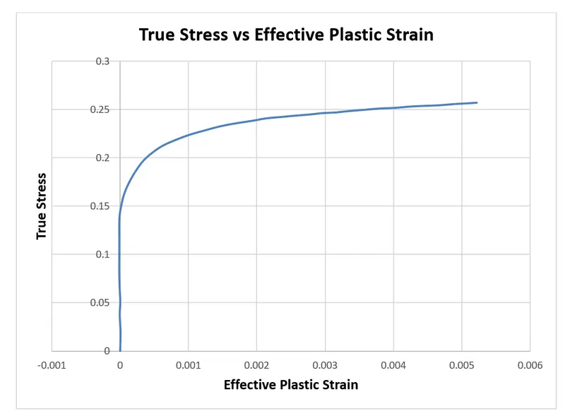
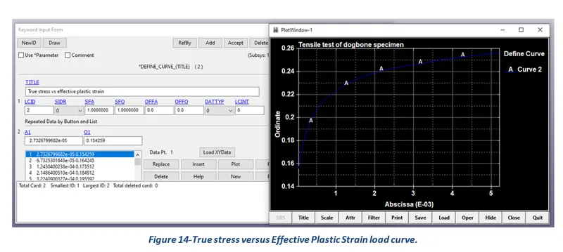
Since LS Dyna does not accept negative values for the Load Curve parameter, therefore the following curve can only be used for the challenge purposes.

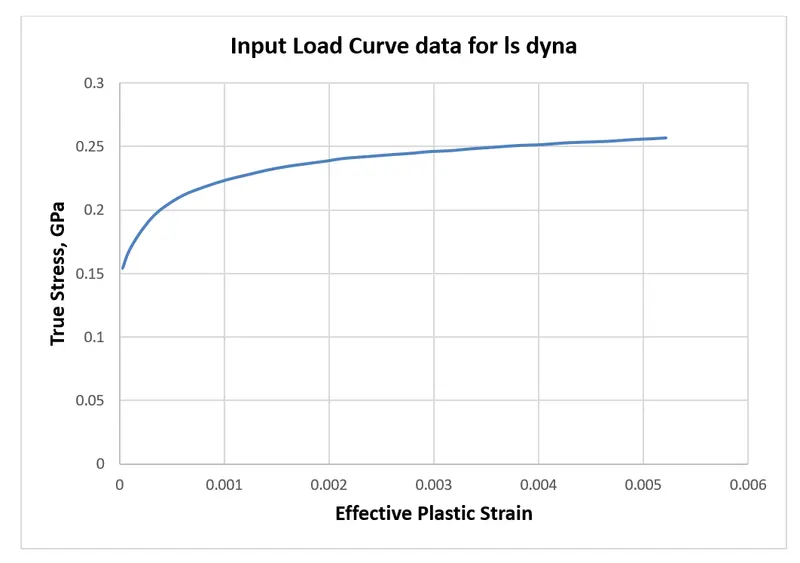
What follows hereafter is the set of images representing the process followed to create different cards and values assigned to their key parameters.

Boundary:

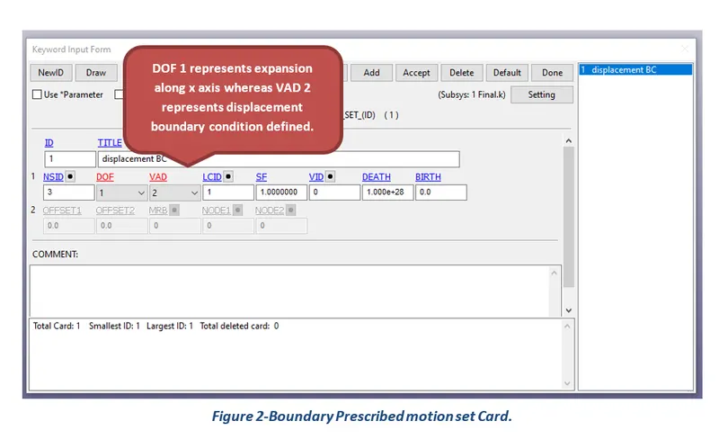
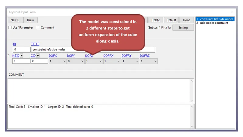
The keyword BOUNDARY provides a way of defining imposed motions on boundary nodes. The Prescribed Motion Set Displacement boundary condition was defined for the challenge purposes. Also, the SPC Set (single Point Constraint) boundary condition was used to restrict the motion of the nodes.

Control:

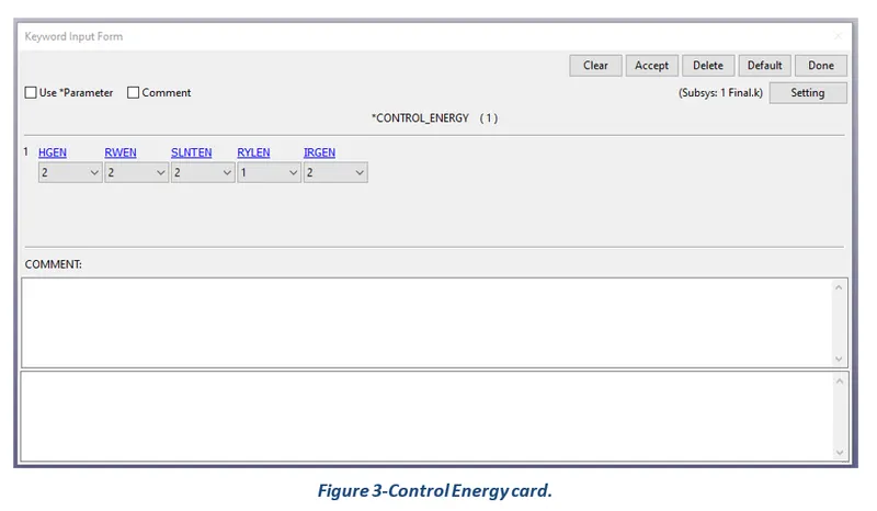
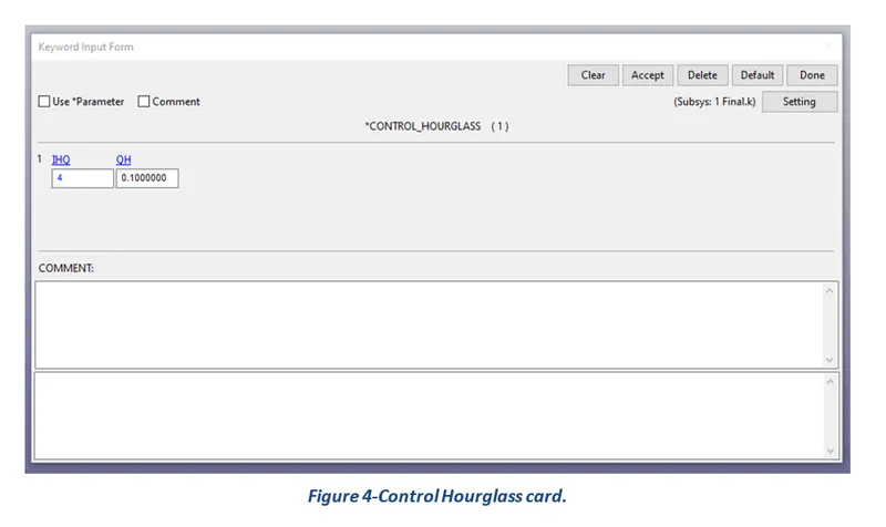
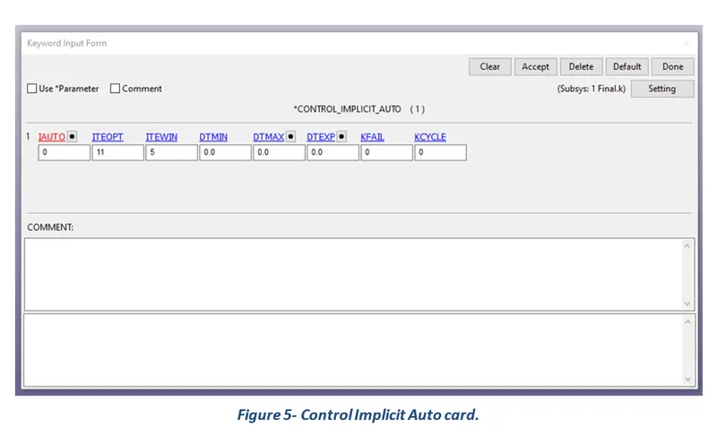
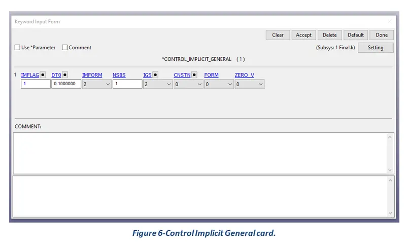
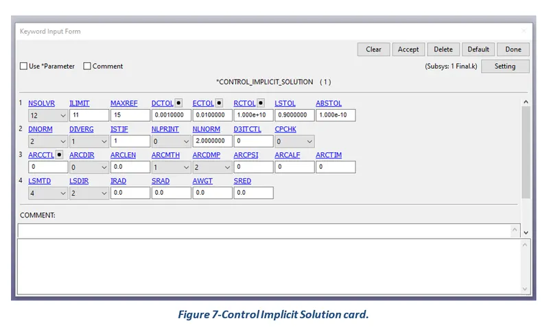
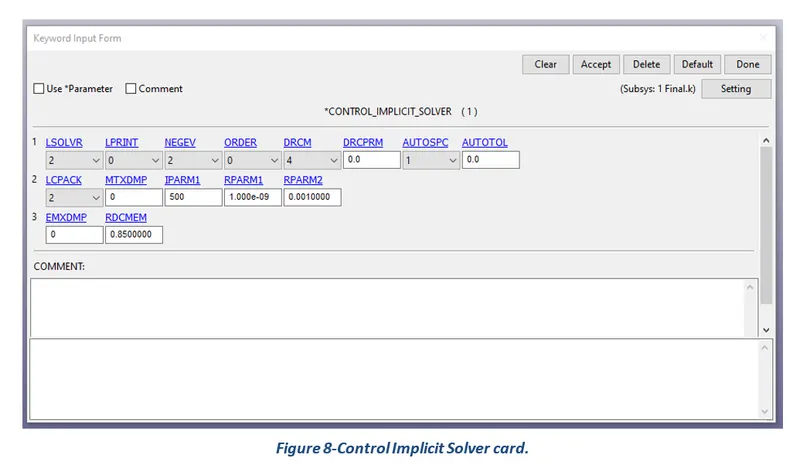
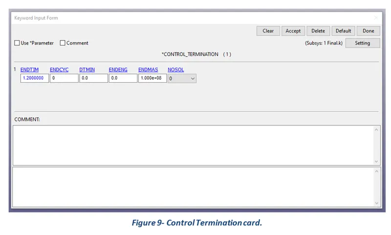
The keyword control cards can be used to change defaults. The control energy, hourglass, implicit auto, implicit general, implicit solution, implicit solver, and control termination cards were created for the challenge purposes.

Database:

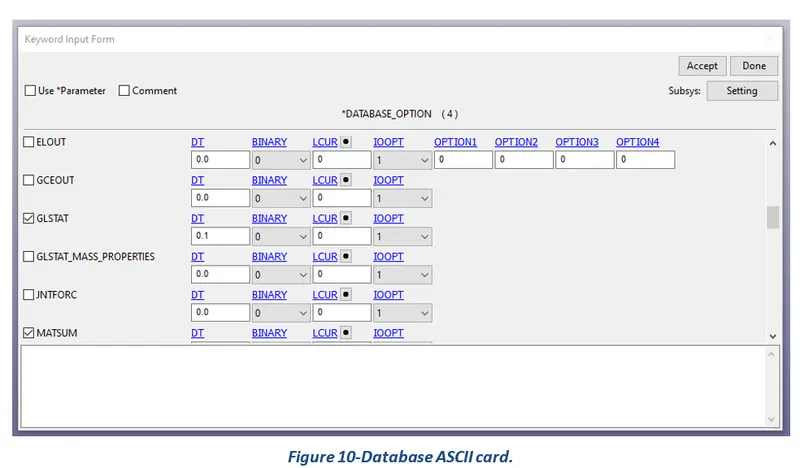
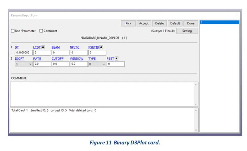
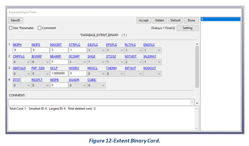
The database definitions are necessary to obtain output files containing results information. The binary D3Plot, Extent Binary, and ASCII options were selected for the challenge purposes.

Define:

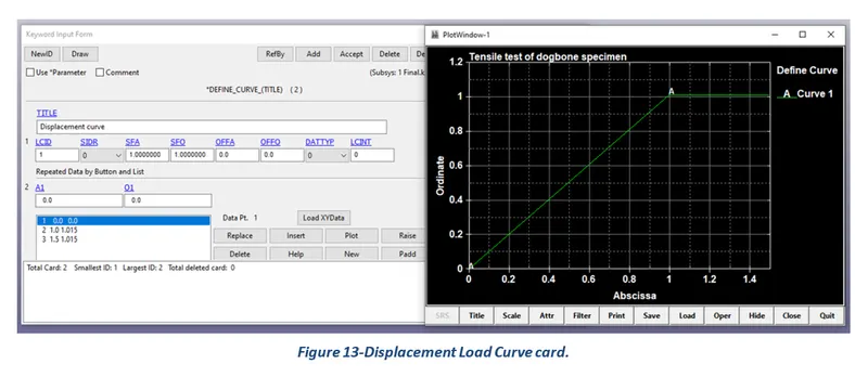
The keyword DEFINE provides a way of defining boxes, coordinate systems, load curves, functions, tables, transformations, and orientation vectors. The curve option was selected, and the assigned value of load-displacement is presented in the following card.

Hourglass:

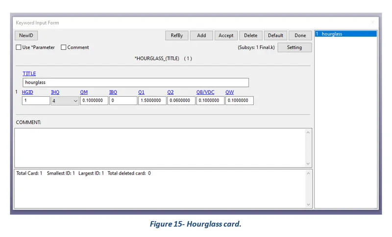
Hourglass (HG) modes are nonphysical, zero-energy modes of deformation that produce zero strain and no stress. Hourglass modes occur only in under-integrated (single integration point) solid, shell, and thick shell elements.

Mat:

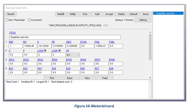
The keyword MAT helps in defining and assigning different types of materials to a part as per requirements. For this challenge MAT 024 Piecewise Linear Plasticity was selected and the values assigned to material card parameters are presented in the following card.

Section:

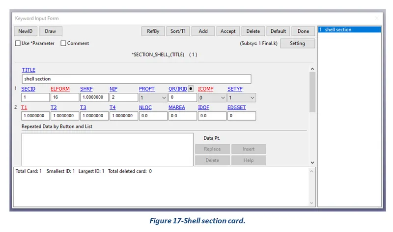
Under section, the element formulation, integration rule, nodal thicknesses, and cross-sectional properties are defined. A solid section was created as per challenge requirements and assigned values for their parameters are presented in the following picture.

Part:

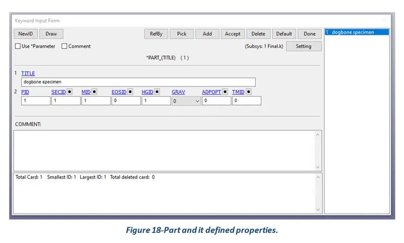
Here define combine material information, section properties, hourglass type, thermal properties, and a flag for part adaptivity.

4 Results

After setting up the input deck and saving the file. K format, the first and foremost step is to perform a model check and then run the simulation using LS-Run software. Once normal termination is achieved, the results can be viewed and analyzed using LS-PrePost software.

Results of uniaxial expansion test of dog bone specimen

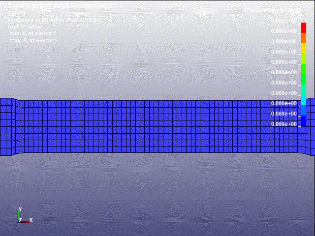
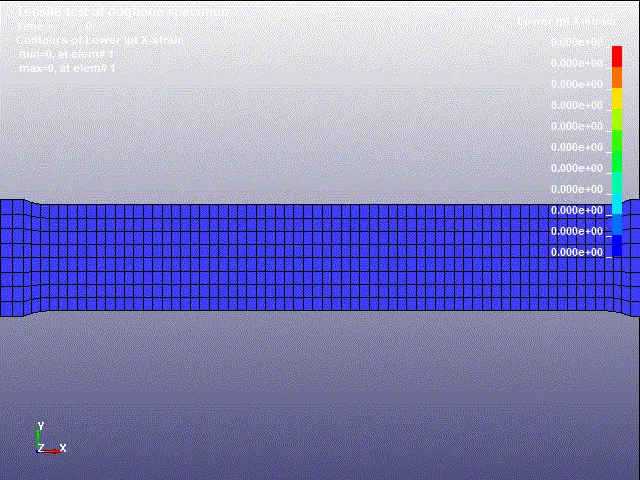
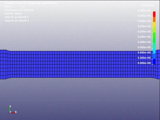
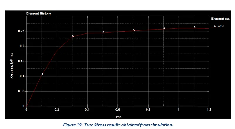
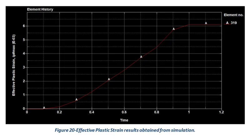
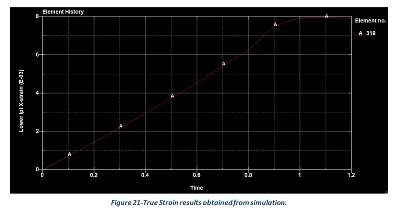
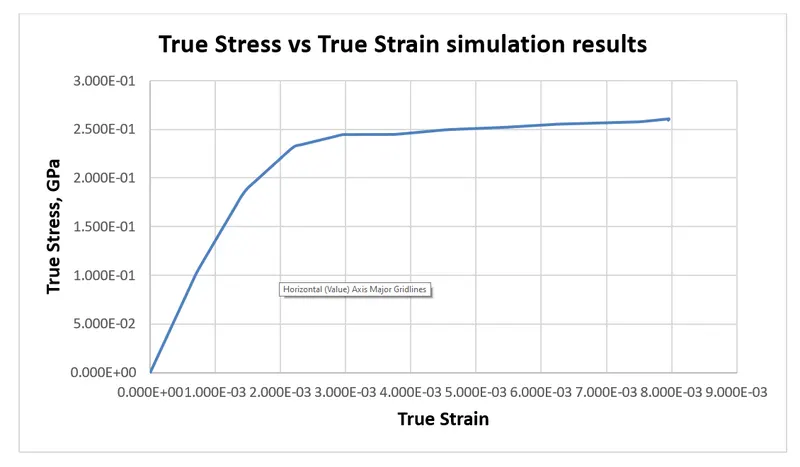
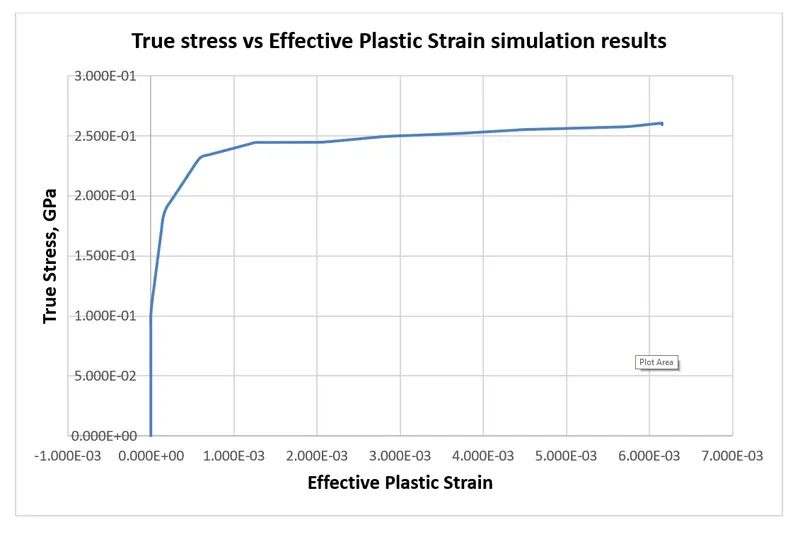
The following graphs present the experimental data for true stress, true strain, and effective plastic strain obtained from running the uniaxial tensile simulation of the dog bone FEA model.

5 Conclusion

The main aim of the Week 9 challenge was to model a MAT 024 Piecewise Linear Plasticity material card from the given true stress/ strain raw data and use it to perform a uniaxial tension test of the given dog-bone specimen and also validate the post-processing stress-strain results with the given raw data. It was observed that the stress-strain curves obtained from the uniaxial test simulation almost behave in a similar fashion as of the given raw data for the challenge. However, the yield point slightly varies for the obtained simulated curves in comparison with the actual given raw data. this could have happened either due to improper modeling of material card parameters (such as density, poisons ratio, etc) or mesh still requires some refinement.