Week - 9 Material Modeling from Raw Data

Skill-lync assignment 9

Aim: The objective of this assignment is to obtain material behaviour data for the given material and use this data to simulate tensile test on the given component, so that the specified material behaviour can be replicated and hence verified.

Case setup: The stress vs. strain plot for cast iron is given for verification, as shown below.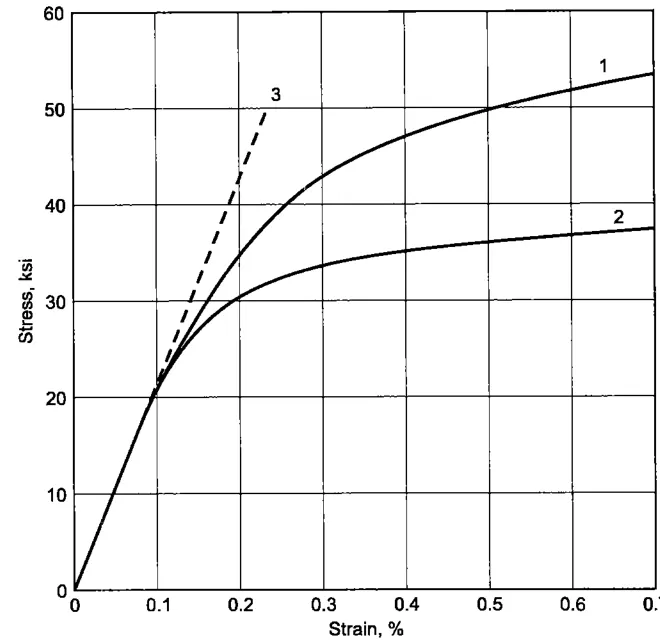

Figure 1: Stress vs. strain plot for cast iron

It shows plots for 2 structures of the same material. The plot 1 is chosen for this assignment.

The component provided is a dog-bone specimen 145 mm long, as shown below, that is supposed to be assigned the given material.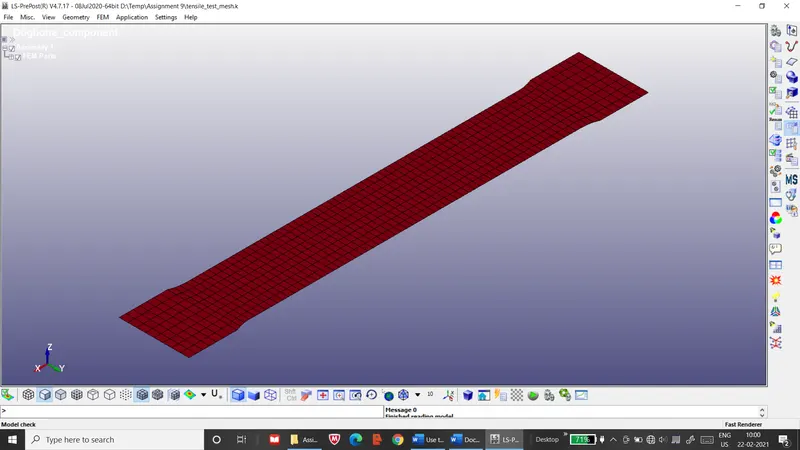

Figure 2: Dog-bone specimen

Procedure: The component and the material are worked on through the following series of steps.

1. The plot image is loaded into a data digitizing software and 108 data points are extracted from the plot and compiled in an excel spreadsheet.
2. The slopes between consecutive data points are calculated and the average of the first 22 slopes is calculated to obtain the Young’s modulus for the material. Beyond this range of data points (up to 0.8% strain), the plot becomes non-linear.
3. The stress values are converted to the kg, mm, ms units and the plastic strain value is derived by subtracting 0.002 (maximum elastic strain) from the total strain. The plastic strain values greater than 0 and their corresponding stress values are saved in a separate excel spreadsheet.
4. The dog-bone component is imported into the LS-PrePost workspace.
5. A section is defined for the component with a thickness of 5 mm and default element formulation of 2 (Belytschko-Tsay).
6. The material curve is defined through the DEFINE_CURVE keyword, where the data is imported from the excel spreadsheet in the following form.

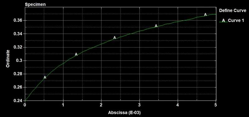Figure 3: Material curve

7. Based on the material curve and literature, the MAT24 (piecewise linear plasticity) material is defined for the component with density of 7.8 X 10^-6 kg/mm3, Young’s modulus of 150 GPa, Poisson’s ratio of 0.33, yield stress of 0.24 GPa and stress curve defined earlier.
8. Constraints are defined such that one end of the component is fixed and the other is free to move in the x-direction.
9. A linear displacement curve is defined for the component up to 1.015 mm (0.7% total strain) at a time of 200 ms. This displacement curve is applied to the moving end of the component.
10. Implicit solver is set by including the CONTROL>IMPLICIT_GENERAL keyword with an initial time step of 1 ms and a run time of 200 ms.
11. The CONTROL>HOURGLASS keyword is included to control hourglass energy generation during simulation and the CONTROL>ENERGY keyword is included to record the hourglass energy produced.
12. The DATABASE>ASCII_option keyword is edited so that glstat file is output from the simulation for post-processing.
13. The file is then saved and run in the LS-Run solver and the resultant d3plot file is imported into the LS-PrePost workspace.
14. The energy history plot is loaded from the glstat file and checked for excess hourglass energy.
15. An element is selected in the middle of the component and its principal stress and strain are plotted separately. These 2 plots are then combined in an X-Y plot to obtain the stress vs. strain plot. This plot is then saved as an excel spreadsheet and compared with the original curve of the material.

Results: The following observations were made from this simulation.

• Energy plot is shown below.

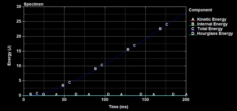Figure 4: Energy plot

It shows normal simulation behaviour with almost no hourglass or kinetic energy. This confirms the accurate element formulation and the quasi-static nature of the simulation.

• The stress vs. strain plot obtained from the simulation is shown below.

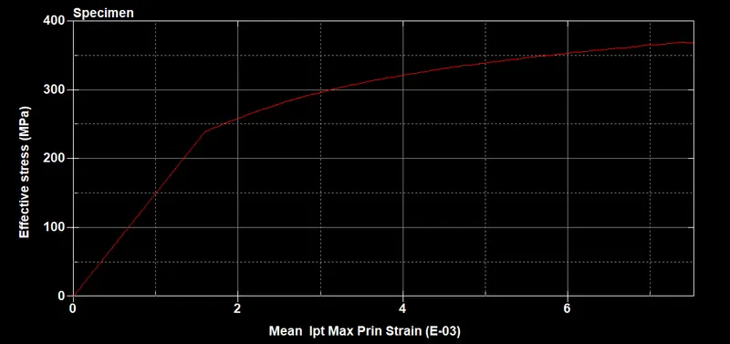Figure 5: Simulated stress vs. strain curve

This curve is compared to the original curve, as shown below.

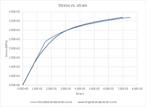Figure 6: Stress curve comparison

It shows that the simulated and original stress-strain curves are almost identical, except around the yield point of the material. This can be accounted for by the limitations of the MAT24 material card. In this card, the material is assumed to have linear elastic behaviour right up to the yield point, which itself was assumed in the simulation to be at the 0.2% strain mark. If the yield point in this material card was set at the end of the linear part of the curve, the simulated curve may resemble the original one better. However, this is not advisable since the material behaviour in negative stresses would be markedly different due to the different yield point, where the material is permanently deformed.

Conclusion: The given material has been successfully implemented in the given component and its behaviour accurately recreated with the adequate material modelling.