Week - 9 Material Modeling from Raw Data
Aim : to perform a material modeling from given graph and verify the same material using dogbone tensile simulation test.
Procedure:
1. open a graph iin Graph digitizer app and find the stress vs strain value on multiple points
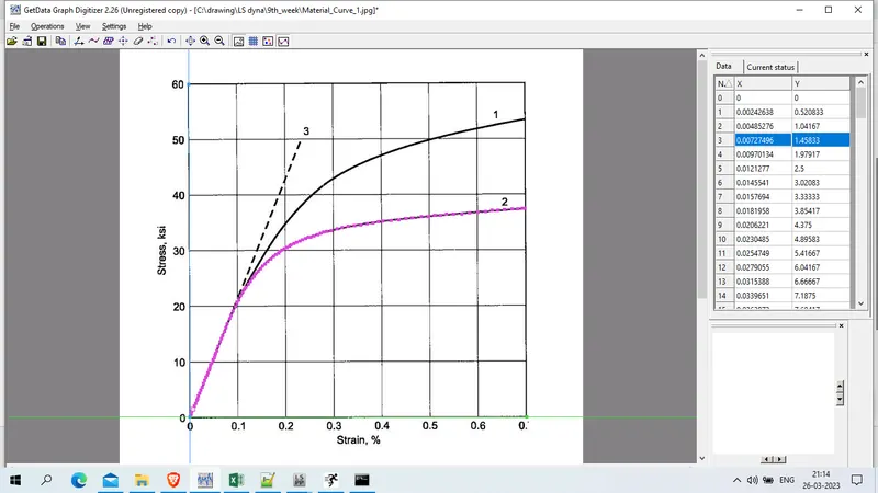
the same extracted value are the true stress and true strain for graphite cast iron material. amd the given stress is in Ksi
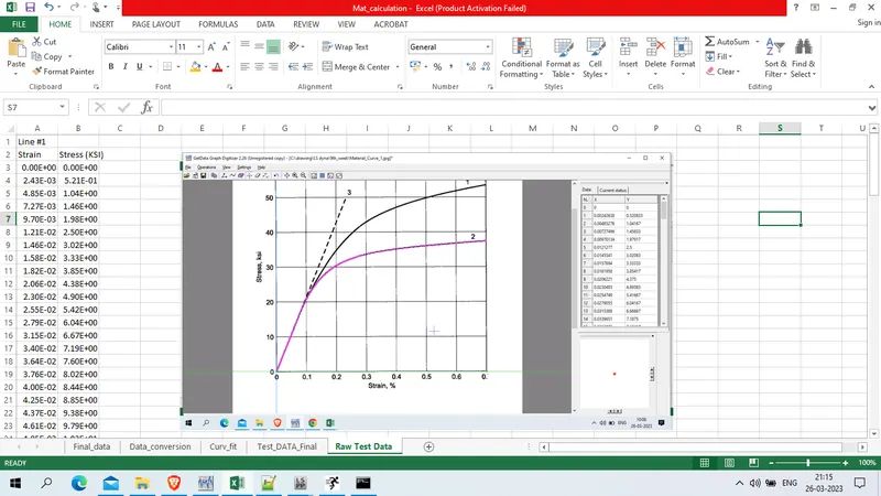
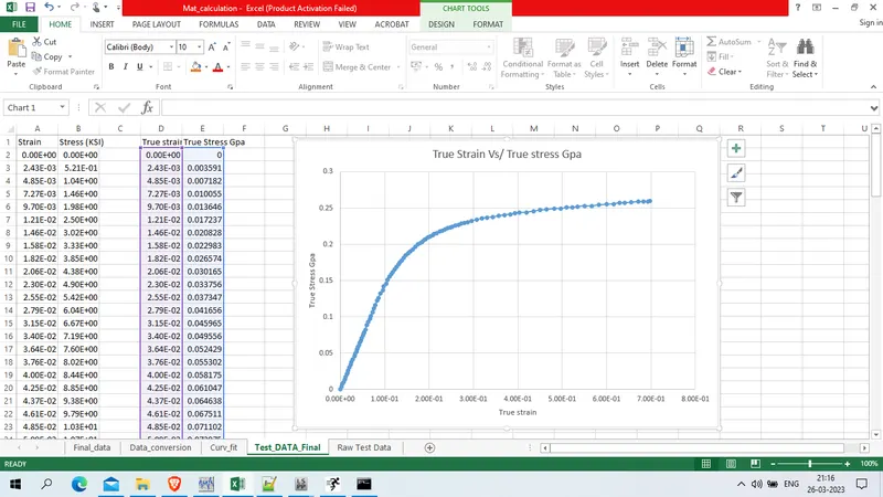
now convert stress values to GPa as we have to use unit system as Kg-mm-ms and the grapg for true stress vs true strain in given below
3. now we will find the yield stress by ploting linear curve with added strain 0.2% as shoen below
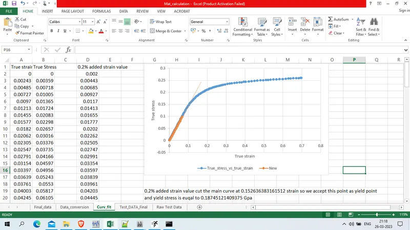
and yield stress is euqal to 0.18745121409375 GPa
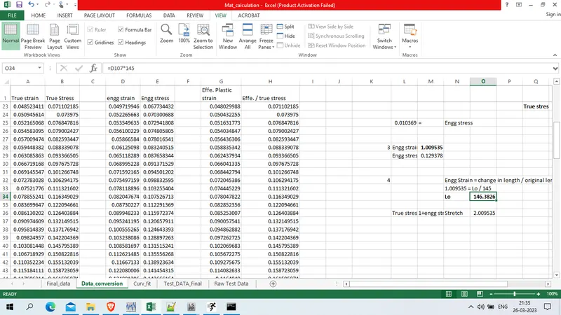
4. now find the engg stress, engg strain , effective plastic strain abd effective plastic stress from the value of truee stress and true strain.\
| True strain | 0.69790 |
| True Stress GPa | 0.25999 |
Engineering strain = EXP(True strain) - 1
= 1.009535
Engineering stress = True stress / Exp ( true strain)
= 0.129378069 GPa
Effective plastic strain = Total true strain - (true stress / E)
where young modulus of Graphite cast Iron (E) = = 20.9E+06 Psi = 144.1 GPa
Effective plastic strain = 0.69609931
Engineering strain = Change in length / Original length
Change in length = 146.34 mm
5. Finally draw a graph after yield point ( plastic zone) with value of effective stress and effective strain
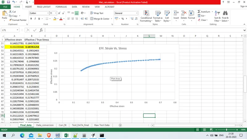
Now material curve is ready for Mat 024 Piecewise_linear_plastic.
now we will open dogbone specimen in LS-prepost
File >> open >> LS DYNA keyword file
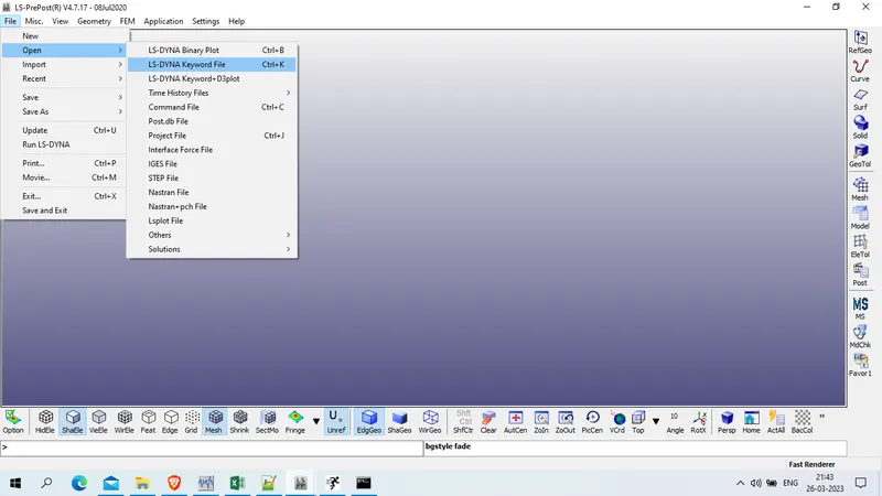
select the file and click on open
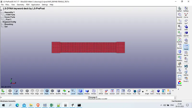
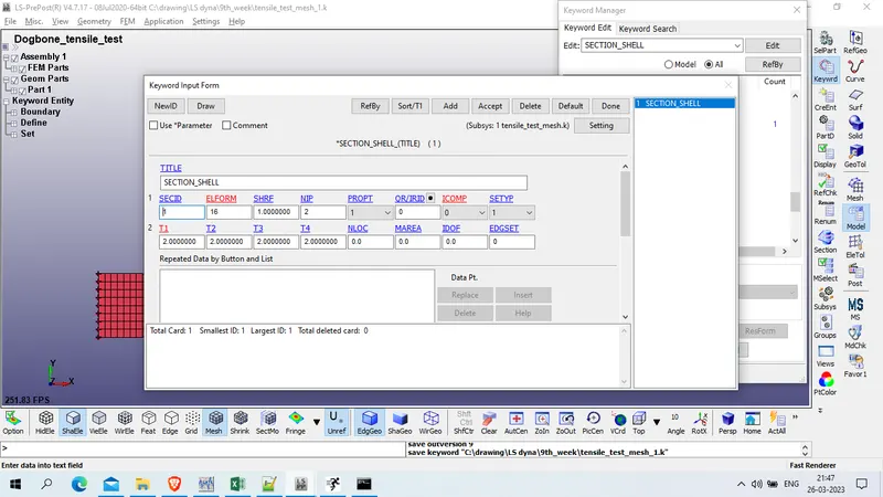
define section_card for this shell element
model and part >> keyword manager >> all >> section >> shell
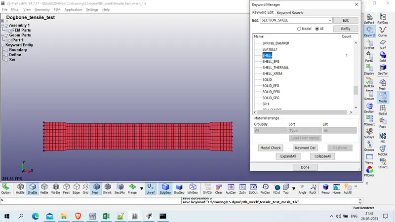
Title : Section_shell
SECID : 1
ELFORM : 16
T1/T2/T3/T4 : 2
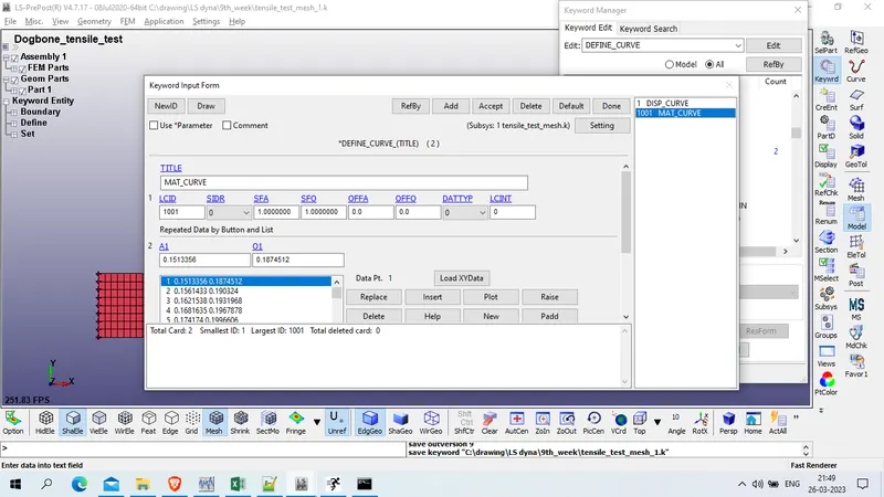
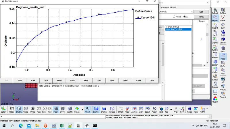
Define material curve
model and part >> keyword manager >> all >> define >> curve
Title : Mat_curve
MID : 1001
define mat card for this specimen
model and part >> keyword manager >> all >> mat >> 024_piecewise_linear_plastic
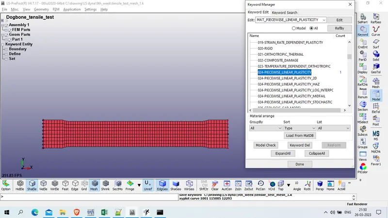
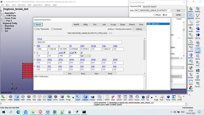
Title : MAT_GCI
MID : 1000
RHo : 7.1E-6 Kg/mm^3
Young's modulus E : 144.1 GPa
Poission Ratio PR : 0.27
Yeild stress : 0.1874512 GPa
provide LCSS : mat_curve
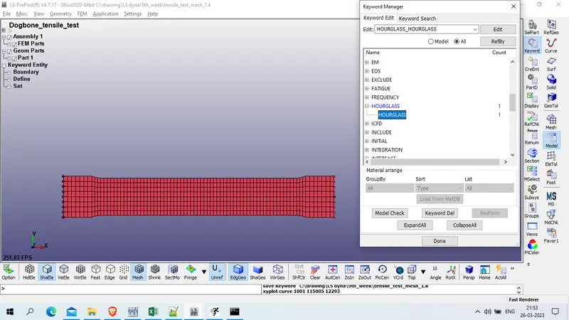
Define Hourglass card
Model and part >> Keyword manager >> all >> hourglass >> hourglass
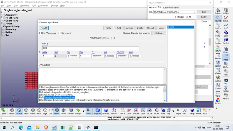
Title : HGL
HGID : 1
IHQ:=Hourglass control typ : 2 (Flanagan-Belytschko viscous form,)
now define Section, Mat and hourglass to part card
Model and part >> keyword manager >> model >> part >> part
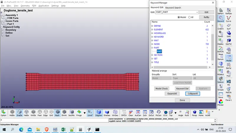
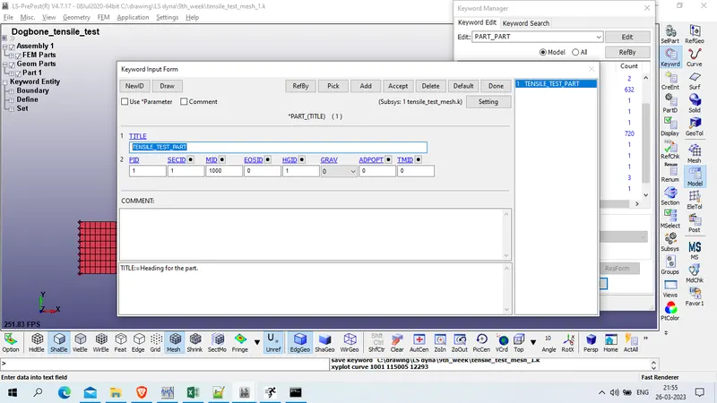
Title : TENSILE_TEST_PART
PID : 1
Now we will define boundary condition for analysis
1st create node set
model and part >> create entity >> set_data>> Set_node
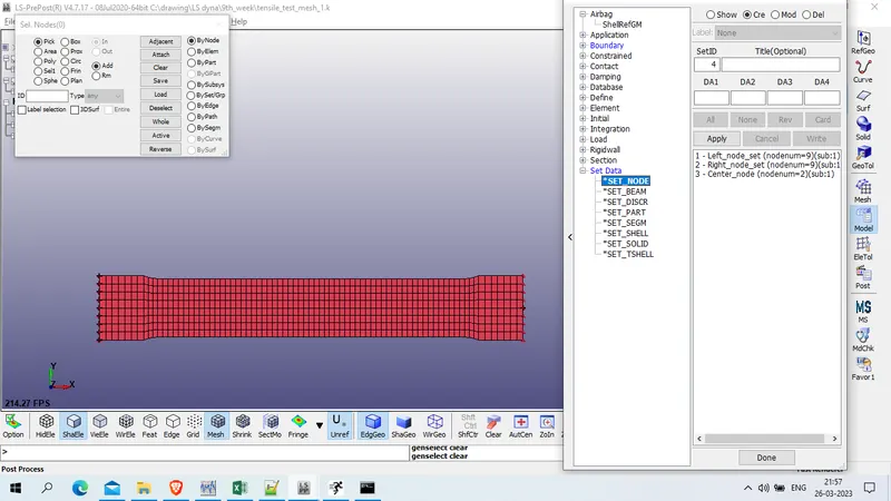
click on create >> select left side node to fix in x and z axis
Title : left Node
select node as shown below
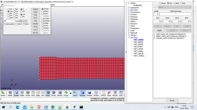
Apply
now select right node and create new node set
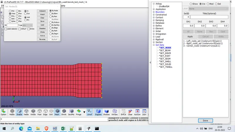
and select 2 node at center to fix in Y axis movement
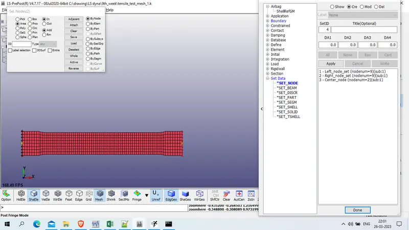
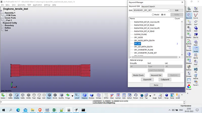
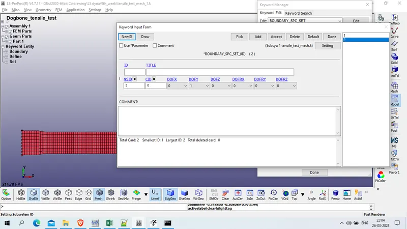
Now define boundary condition for that
model and part >> keyword manager >> boundary >> SPC_set
Node ste id : 1
DOF X and DOX Z : 1
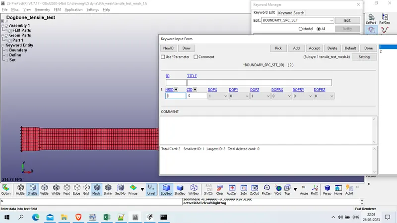
Node set Id : 3
DOF Y : 1
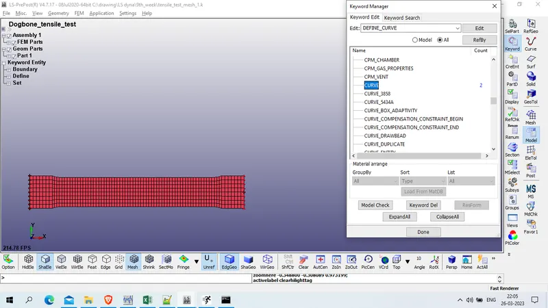
Now create curve for displacement
Model and part >> keyword manager >>all >> Define >> curve >> add
Title : DISP_CURVE
LCID : 1
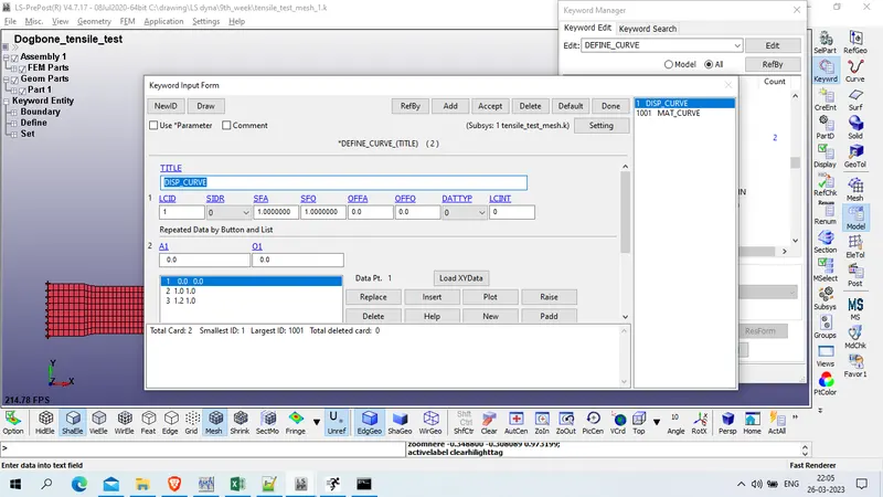
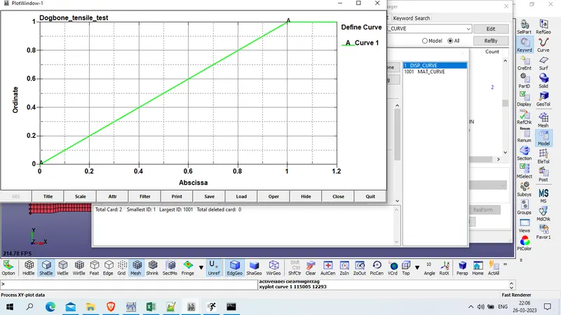
Now define prescribe_motion_displacement
Model and part >> keyword manager >> all >> baundary >> prescribe _motion_set
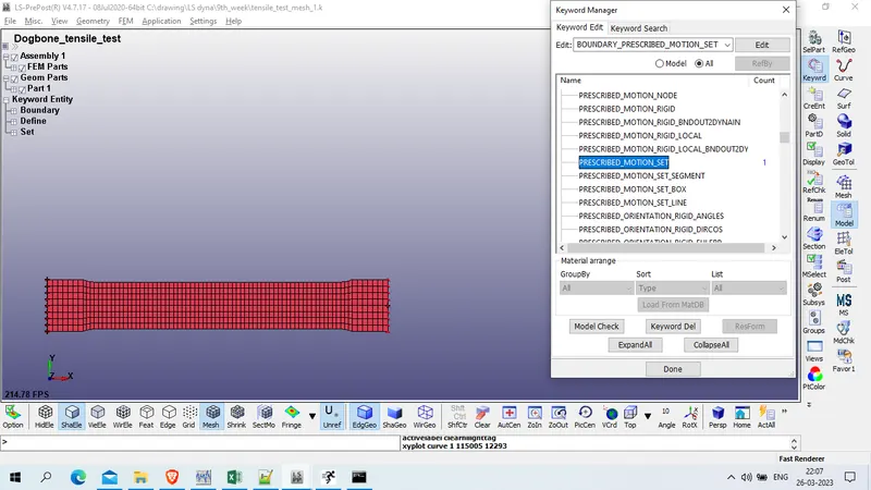
select
NSID : node set id : select right node set : 2
DOF : 1 ( x displacement )
VAD : 2 ( displacement )
LCID :1
SF : 147
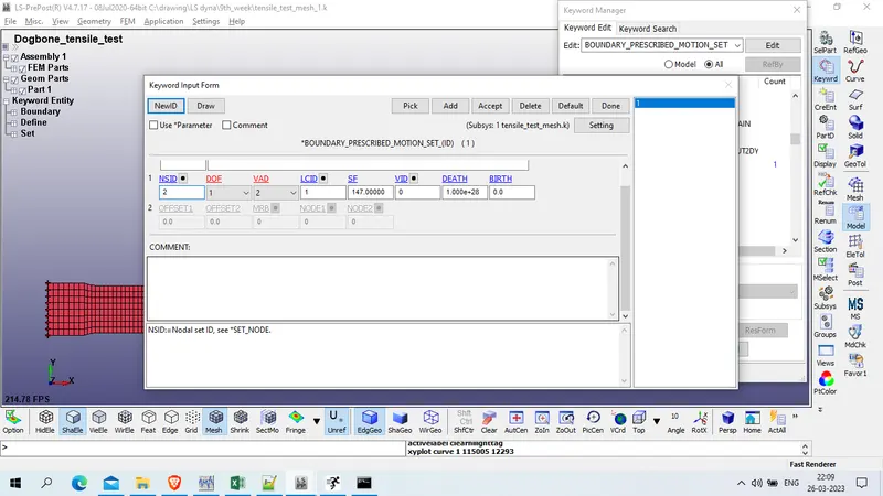
Define control_energy card
model and part >> keyword manager >>all >> control >> energy
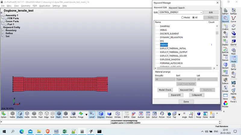
HGEN:=Hourglass energy calculation option. : 2: hourglass energy is computed and included in the energy balance.
RWEN:=Stonewall energy dissipation option:2: energy dissipation is computed and included in the energy balance (default).
SLNTEN:=Sliding interface energy dissipation option: 2: energy dissipation is computed and included in the energy balance.
RYLEN:=Rayleigh energy dissipation option (damping energy dissipation):2: energy dissipation is computed and included in the energy balance.
IRGEN:=2: initial reference geometry energy is computed and included in the energy balance as part of the internal energy (default).
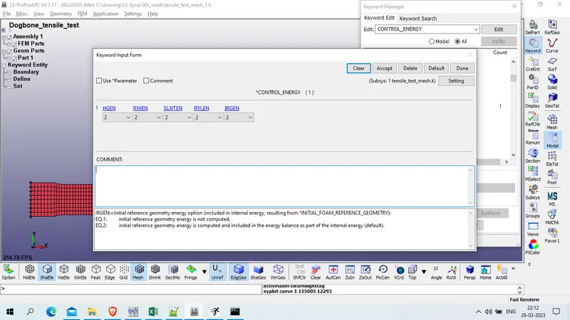
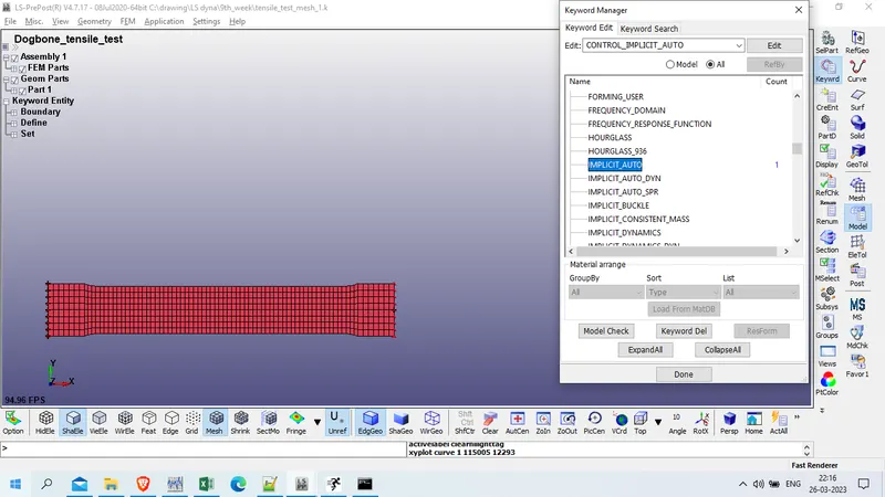
activate implicit solver by introducing implicit auto, implicit general and implicit solver card
Model and part >> keyword manager >> all >> control >> implict_auto
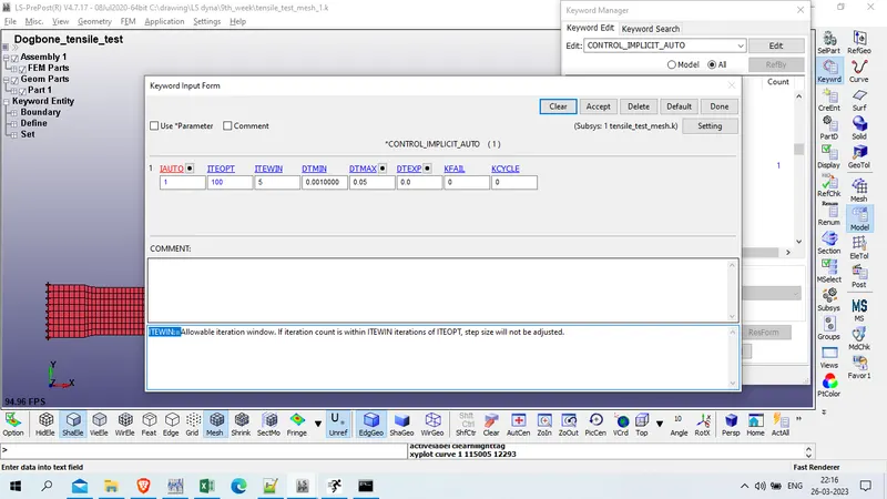
IAUTO: 1
ITEOPT : 100
ITEWIN:=5
dtmin : 0.001
Dtmax : 0.05
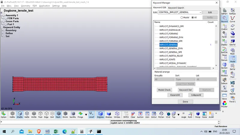
for implicit general
Model and part >> keyword manager >> all >> control >> implicit_general
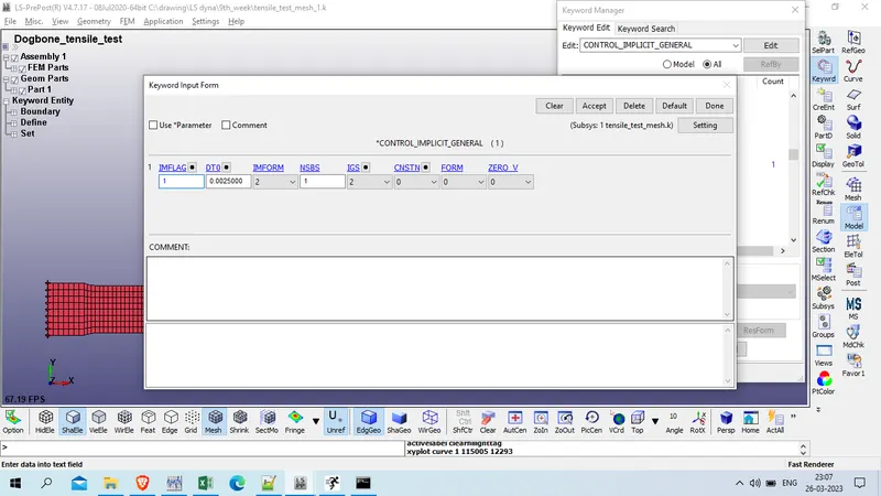
Imflag : 1
DTO : 0.0025
IMform : 2
for implicit solver
Model and part >> keyword manager >> all >> control >> implicit_solver
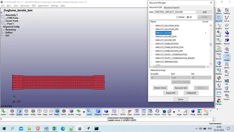
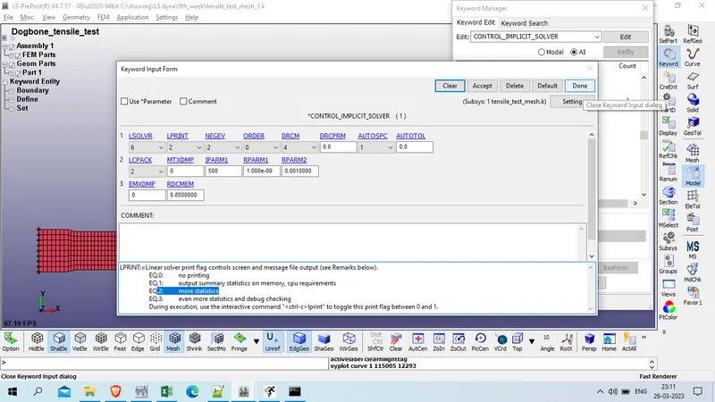
LSOLVR : 6: BCSLIB-EXT, direct, sparse, double precision
LPRINT : 2: more statistics
Now define database card for output
Define BINARY_D2Plot
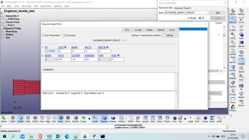
Model and part >> Keyword manager >> all >> database >> BINARY_D3Plot
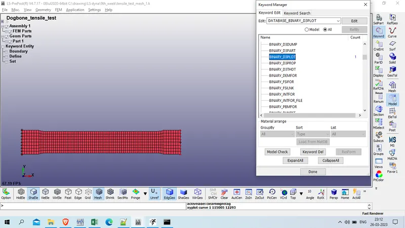
DT : 0.01
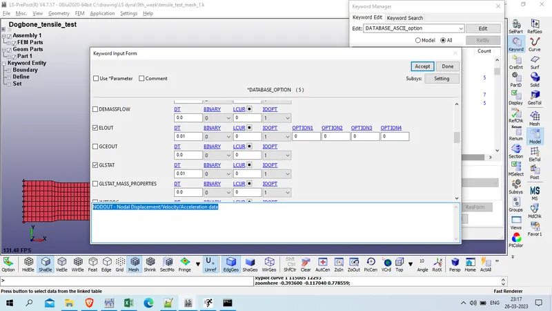
ASCII_OPTION Card
define below output
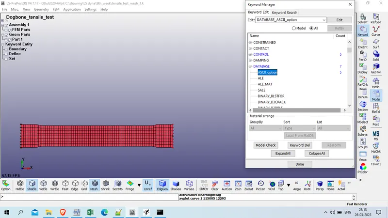
ELOUT - Element Output Data
GLSTAT - Global Statistics
MATSUM - Material Energies
NODOUT - Nodal Displacement/Velocity/Acceleration data
with DT : 0.01
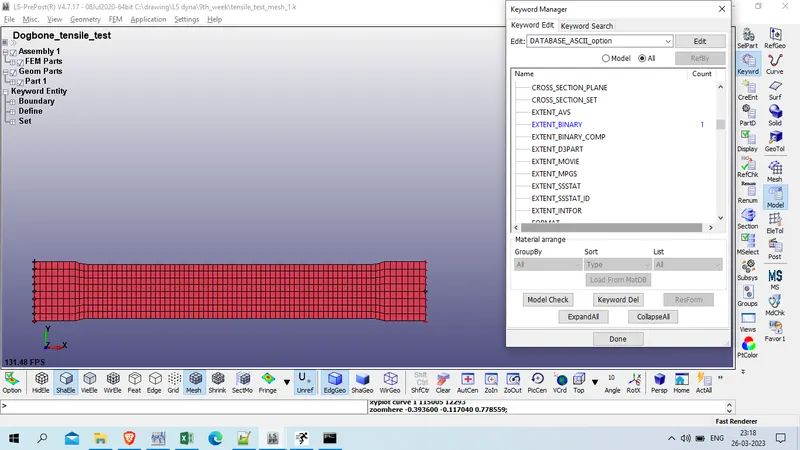
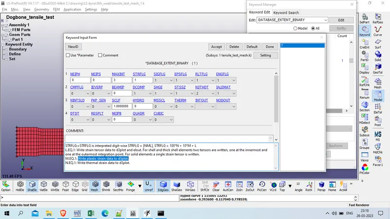
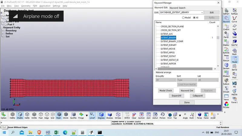
EXTEND BINARY Card
Model and part >> Keyword manager >> all >> Database >> Extend_BINARY
STRFLG: 1 Write plastic strain data to d3plot.
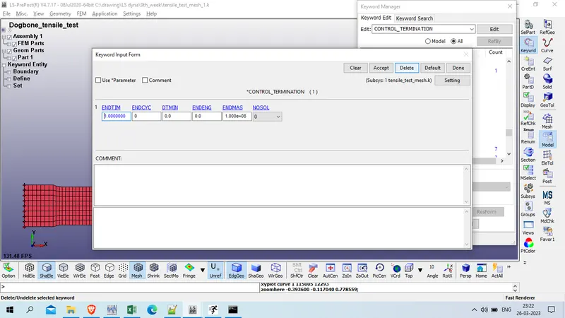
Define termination card
model and part >> keyword manager >> all >> control >> termination
ENDTIM : 1
now check for keyword error
model checker >> keyword check >> recheck
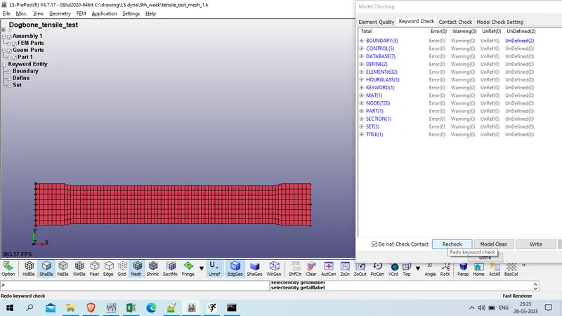
as we have zero error we will procedd for save this file and run the simulation
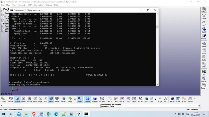
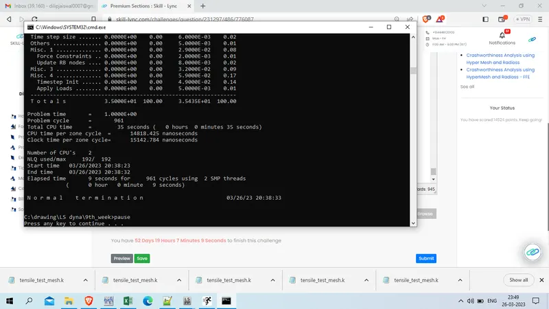
Result :
Von-Mises stress
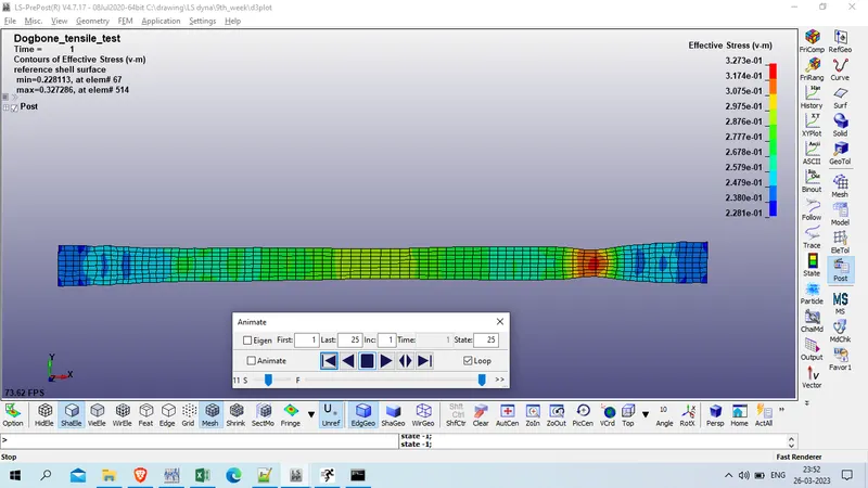
The maximum Von mises stress
Effective plastic Strain
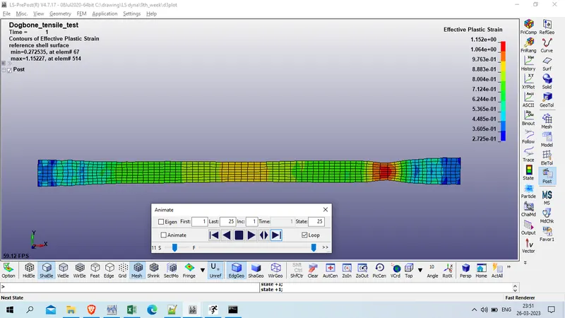
Von mises stress experiance by the element no 503 is given as below
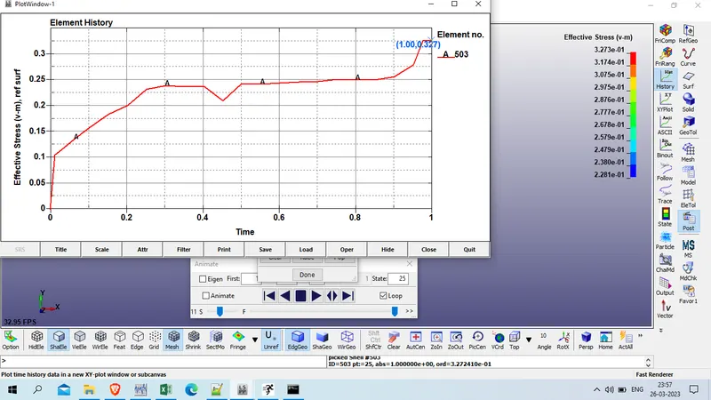
The max von mises stress experiance by element no 503 0.327 GPa.
Effective plastic strain experiance by element no 503 is given as below
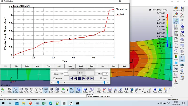
Max effective plastic strain is 1.15 mm
Von misses stress vs. Effective plastic strain graph as per given below
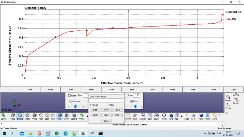
The curve exactly fits the experimental data.
Conclusion : Thus the tensile test is performed on the given dogbone specimen and the simulated values of true stress and strain are validated with the experimental data.