Week - 9 Material Modeling from Raw Data
OBJECTIVE
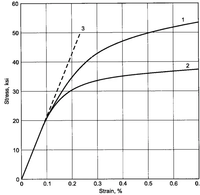
- Use graph digitizer to extract data point of True Stress vs True Strain of anyone graph given below.
- Use these data points and Create a MAT24_PIECEWISE_LINEAR_PLASTICITY material card for an elastic-plastic material
- Verify the material card by performing a uniform tensile test on a dogbone specimen
THEORY
- Material modelling plays an important role in determining the accuracy of simulation results and thus it is a very important task in CAE industries. The team works on extracting the data from actual experiments or past available resources and turns them into solver-accepted material cards.
- Usually, multiple tests are done and the data obtained from these tests are either averaged out or the best data curve is taken up for further processing. Around 150 to 200 data points are selected as raw data. The raw data is filtered off of the noise present.
- Now the data obtained after processing is usually taken as a curve input for material cards. We will follow a similar procedure for our exercise.
PROCEDURE
Data Extraction
- We have two graphs of true stress vs true strain for graphite iron casting with different structures. Select the curve ‘1’ as our study input.
- Now use Graph digitizer to get the data points from the graph. These data points are copied to excel.
Data Cleanup
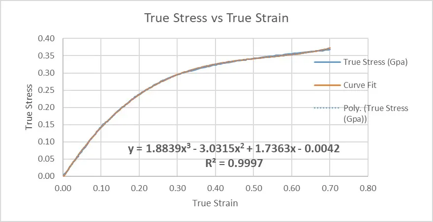
- Create a graph using these data points. Go to the trendline option and select a polynomial option to get a closer trendline. Change the power option to identify a closer trend.
- Use this trendline equation and generate the stress data for the same strain
Data conversion
- Since our data is in ksi, we require our data in kg-mm-ms unit. Use unit conversion to get the value of stress in the required unit system.
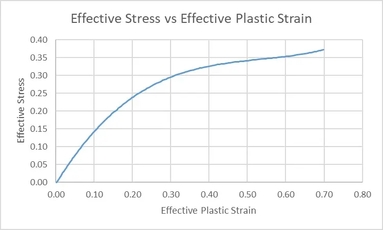
- Since we are modelling an elastic-plastic material, our main concern is the plastic zone of the material. So instead of engineering stress-strain data, we will convert our data in Effective Stress vs Eff Plastic Strain data using the following formulae
Effective Stress = True Stress
Effective Plastic strain = True Strain – (True Stress/E), E = 20.9e+6 psi
Curve
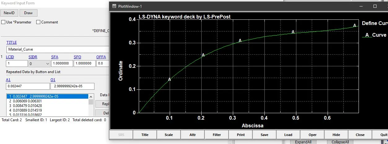
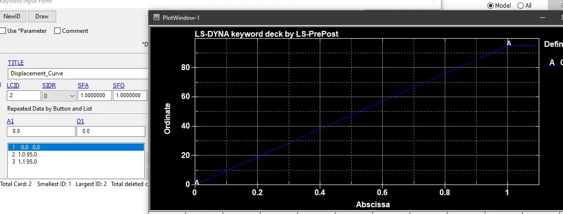
- Create 2 curves. One curve defines the displacement of the specimen and another cover to define the material stress-strain property
Part, Section and Material Card
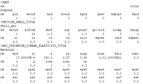
- Here we will use the MAT24 card to create the material card.
- Input the values of density, poisons ratio and yield strength as below. Also for defining the plastic region we will use the above curve instead of tangent modulus.
- Create a shell section for the specimen.
- Assign section id and material id to the part.
Boundary conditions
- Here we are performing a uniaxial tensile test on a dogbone specimen.
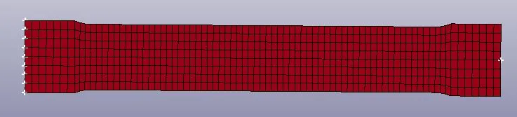
- Constrain all the nodes of the left side in all directions. Also, select the mid node of the extreme left and extreme right and constrain its motion in the Y direction to restrict any slip in the specimen.
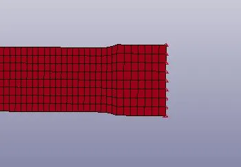
- Create a Boundary_Prescribed_Motion_Set to define the displacement on the nodes on the extreme right end as shown below.
Control
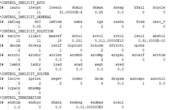
- Since this is a static simulation and we are concerned with the only end result, we will be proceeding with this activity using implicit simulation.
- We will use CONTROL_IMPLICIT_GENERAL, CONTROL_IMPLICIT_AUTO, and CONTROL_IMPLICIT_SOLUTION AND CONTROL_IMPLICIT SOLVER to define the solver type and time step info.
Database
- Use d3plot to write the output of the simulation
RESULT
- Below images show the stress and strain distribution in the specimen
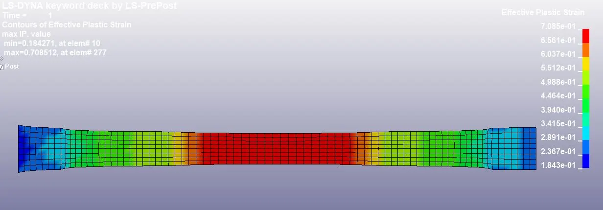
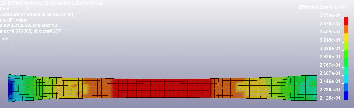
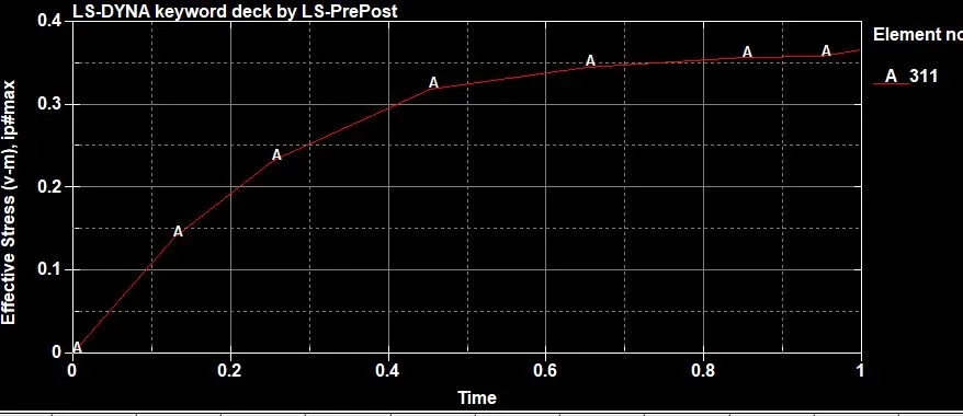
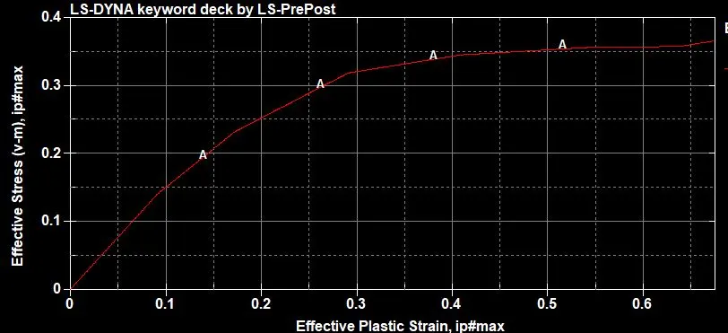
- The stress and strain are as follows.
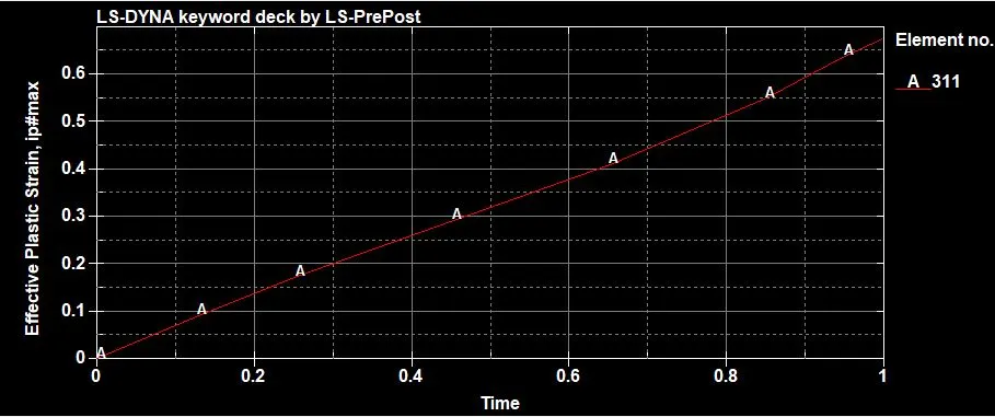
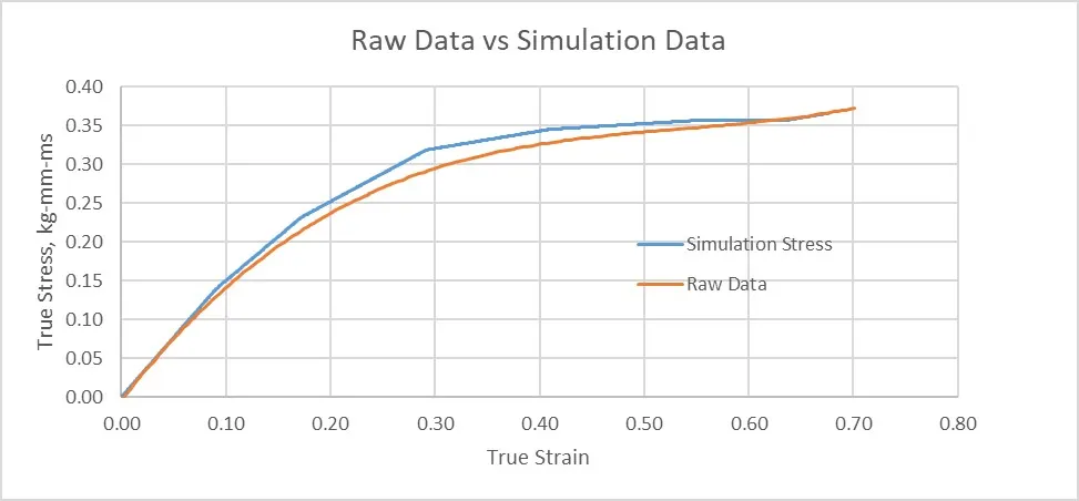
- The True stress vs True strain from the simulation is compared with that of original data as below. From the graph, we can say that our material model is up to the required accuracy as it almost matched the original raw data. This validates the created material using the raw data curve.
CONCLUSION
- From the above exercise, we learned the process of modeling material in Ls-Dyna from the available test/sample data.
- Also, we saw little variation in the simulation data, which is due to the lack of information like density and Poisson’s ratio for the raw data. This variation can be fine-tuned by trying different values of these properties and by selecting more data points to better capture the curve feature