Assignment 4-RADIOSS Material Laws Challenge

1. Total number of cycles, Energy error, mass error and simulation time.
2. Notice the animation of all 5 and describe the animations in brief on the
basis of whether the elements are being deleted or cracked.
3. Plot energies and notice any difference.
4. Based on all the results, which case would represent the on-field
scenario.
5. Prepare a ppt/docx and list down case by case result and your conclusion
as to why the failure happened.

case 1 :-

Law2_epsmax_failure

step 1 : Import the FAILURE_JOHNSON_0000.rad in Hypermesh solver desk.

step 2 : check the properties and Run the model and save as Law2_epsmax_failure_0000.rad

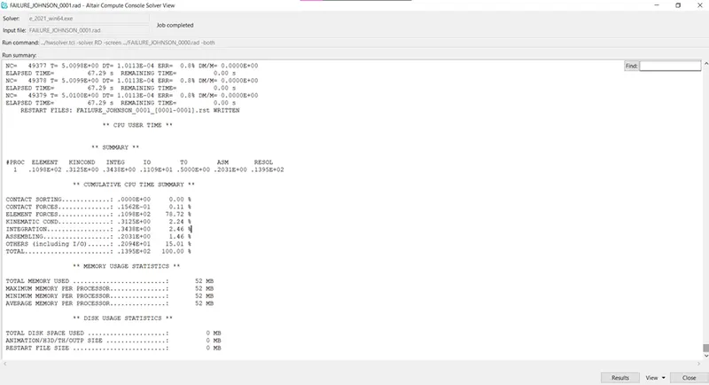
step 3 : Check the file Law2_epsmax_failure_0000.out for no of cycles, energy error, mass error and elapsed time.

Total number of cycles = 49218

Mass error= 0

Energy error = 0.8%

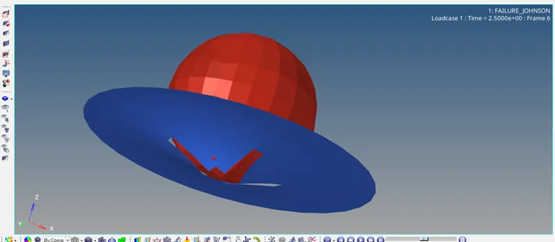
Step 4 : Open the file in Hyperview and open the .h3d file and see the animation of simulation.

Step 5 : open the T.out file in HyperGraph 2D and take the energy graphs.

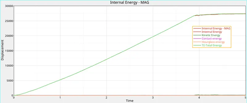
• As per the above graph showing the value of Internal Energy as 26280J and Total Energy as 26349.69J, the increases up to 4ms timestep then becomes constant because of element deletion.
• The Kinetic energy shows some positive value below 2500J but Contact and Hourglass energies are zero, this is because the material card setting with QEPH.

case 2:-

Law2_epsmax_crack

step 1 : Import the Law2_epsmax_failure_0000.rad in Hypermesh solver desk.

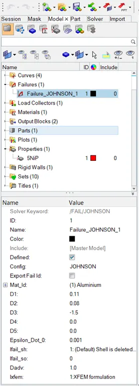
step 2 : check the properties and change the s, Change the values Ifail_sh=1, Dadv=1 and Ixfem=1 in /FAIL/JOHNSON card. Run the model and save as Law2_epsmax_failure_0000.rad.

Here,

Ifail_sh 1 is used for element cracking or deletion
Dadv 1 is used for crack advancement
Ixfem 1 is used for failure criteria for element cracking or deletion

Step 3: Then run the model to separate folder with name as Law2_epsmax_crack_0000.rad. From the out put file checl the values for no of cycles, energy error, mass error and elapsed time

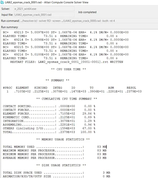
Total number of cycles = 49217

Mass error = 0

Energy error = 4.1%

Step 4 : Open the file in Hyperview and open the .h3d file and see the animation of simulation.

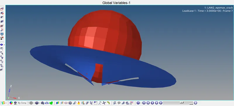
Step 5 : open the T.out file in HyperGraph 2D and take the energy graphs.

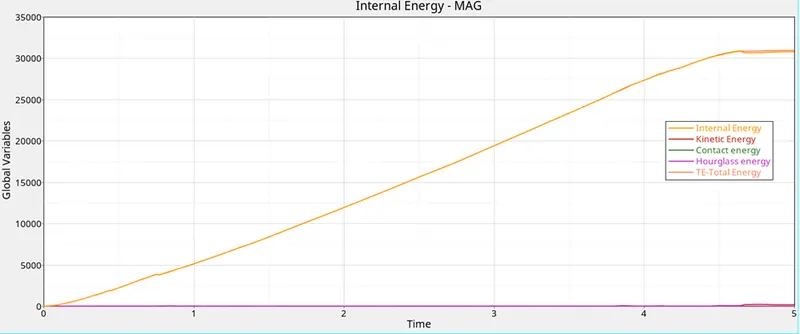
In case we can observe that,

• If you observe the simulation when we add the Ixfem we can see that elements are getting craked as shown in the animation.
• Ixfem is repersented the cark over the elements and it will give more realastic behaviour to the simulation.
• When comming to the graph there both elastic and plastic region is shown in the above graph and having some fluctuating in kinetic and interal energy of elements when they deform.
• If your material model should be very accurate and then the way Ixfem treatment goes it dicipates little more energy and because of that ,for smaller propagation or for local deformations Ixfem could be the good method.
• Ixfem is only used for shell elements only.

case 3:-

step 1 : Import the Law2_epsmax_crack_0000.rad in Hypermesh solver desk.

step 2 : Delet the Failure Jhonson card and Run the model and save as Law_epsmax_nofail_0000.rad.

Step 3: Then run the model to separate folder with name as Law2_epsmax_nofail_0000.rad. From the out put file check the values for no of cycles, energy error, mass error and elapsed time

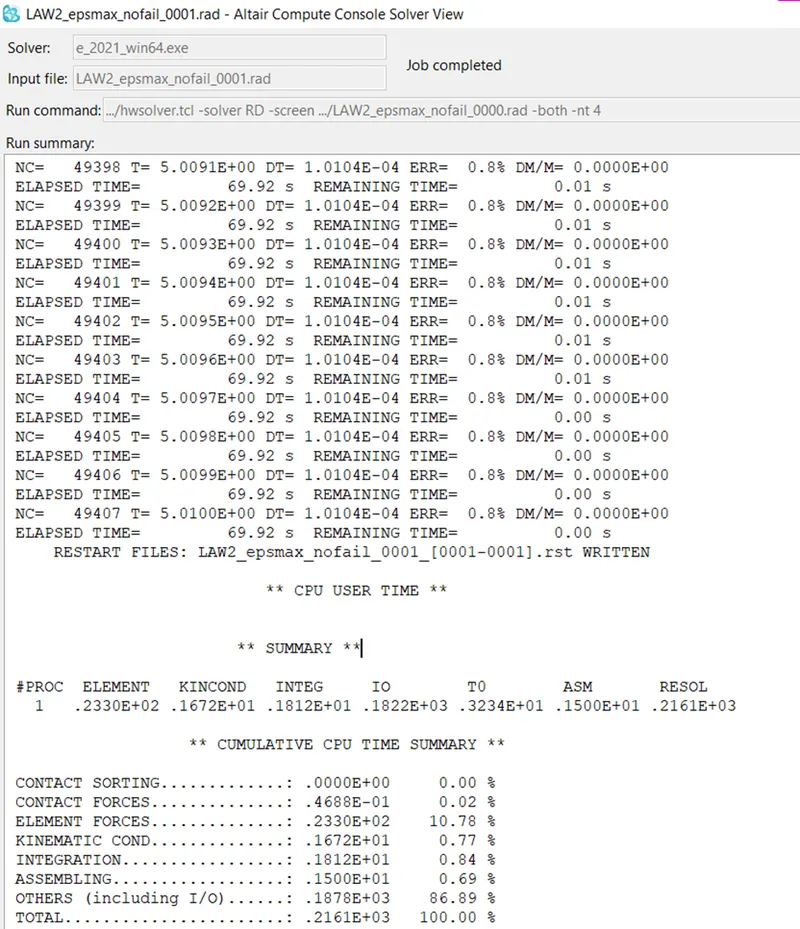
Total number of cycles = 49408

Mass error = 0
Energy error = 0.8%

Step 4 : Open the file in Hyperview and open the .h3d file and see the animation of simulation.

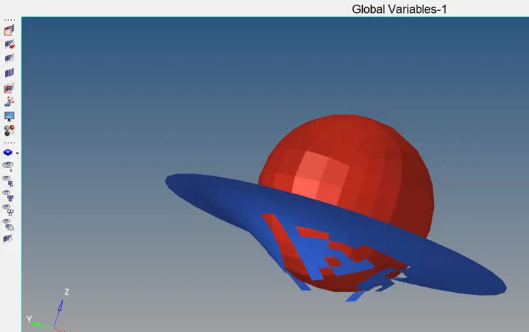
Step 5 : open the T.out file in HyperGraph 2D and take the energy graphs.

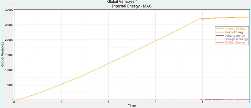
• As we comapre the case1 and case3 there is very small very in the stress .
• But when we are not given the failure card there is directly deformation occurs.
• When comming to the graph there both elastic and plastic region is shown in the above graph and having some fluctuating in kinetic and interal energy of elements when they deform.
• As shown in the above graph the kinetic energy started at zero and at the time of ball hits the surface of the palte the deformation in occurs on the elements then they will obsorb some kinetic energy that fluctuating is shown in the above graph.

case 4:-

step 1 : Import the FAILURE_JOHNSON_0000.rad in Hypermesh solver desk.

step 2 : check the properties and Run the model and save as Law2_epsmax_failure_0000.rad

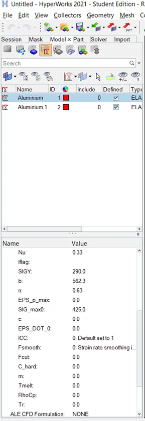
Step 3: Then run the model to separate folder with name as Law2 _0000.rad. From the out put file checl the values for no of cycles, energy error, mass error and elapsed time

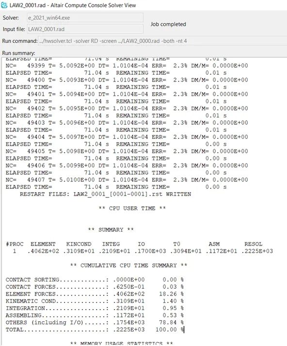
Total number of cycles = 49408

Mass error = 0
Energy error = 2.3%

Step 4 : Open the file in Hyperview and open the .h3d file and see the animation of simulation.

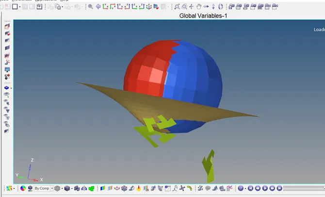
Step 5 : open the T.out file in HyperGraph 2D and take the energy graphs.

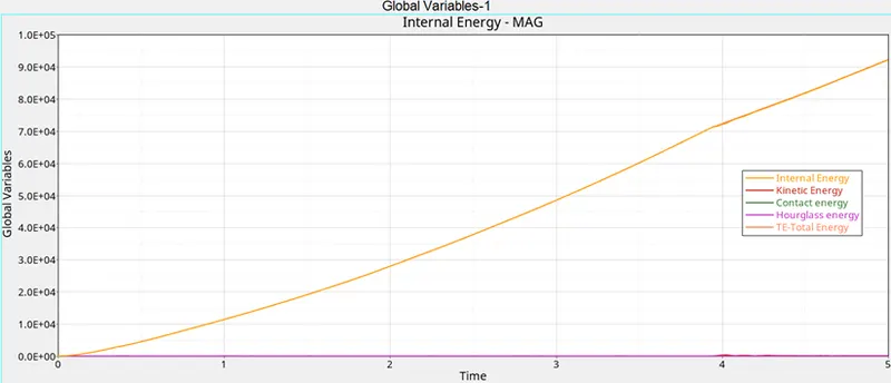
• In case4 here we are deleting the Eps_max value, Eps_max value is the maximum plastic strain for element deletion for any loading (tensile , shear or compression).
• Here we are not given the Eps_max value so that the animation showing that there is direct deletion of elements without cracks.
• As we observe the graph it showing only the elastic region there is a no plastic region that means it breaking happens after the elastic region.

case 5:-

step 1 : Import the e Law2 _0000.rad in Hypermesh solver desk.

step 2 : Check the properties, Change the card to M1_ELAST.

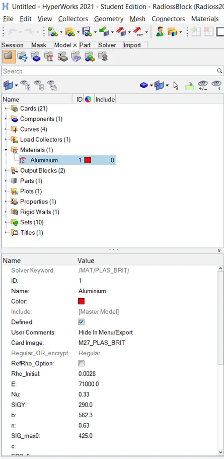
Step 3: Then run the model to separate folder with name as Law1_0000.rad. From the out put file checl the values for no of cycles, energy error, mass error and elapsed time.

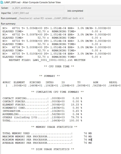
Total number of cycles = 48736

Mass error= 0
Energy error= 3.0%

Step 4 : Open the file in Hyperview and open the .h3d file and see the animation of simulation.

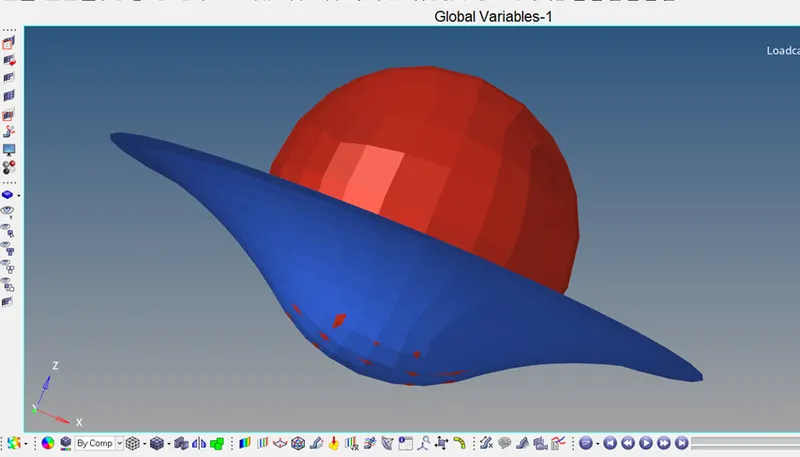
Step 5 : open the T.out file in HyperGraph 2D and take the energy graphs.

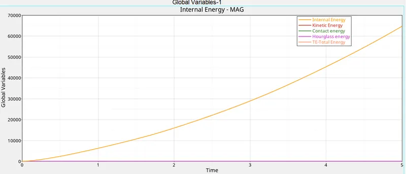
• In case5 we are converting the material model to law1 elastic with the same density,young's modulus and poission ratio.
• As we observe the animation there is no element deletion because it is the an law1 elastic material.
• As we abserve the graph it represents a linear relationship between stress and strain as shown in above graph.
• And there there is no fluctuation of kinetic and internal energy because there is no element deletion here it is purely elastic material
• In this case Deformation is occurs with in the elastic limit .

case 6:-

step 1 : Import the e Law27_0000.rad in Hypermesh solver desk.

step 2 : Check the properties, Card image is M27_PLAS_BRIT with same values of density, Young’s modulus, Poisson’s ratio

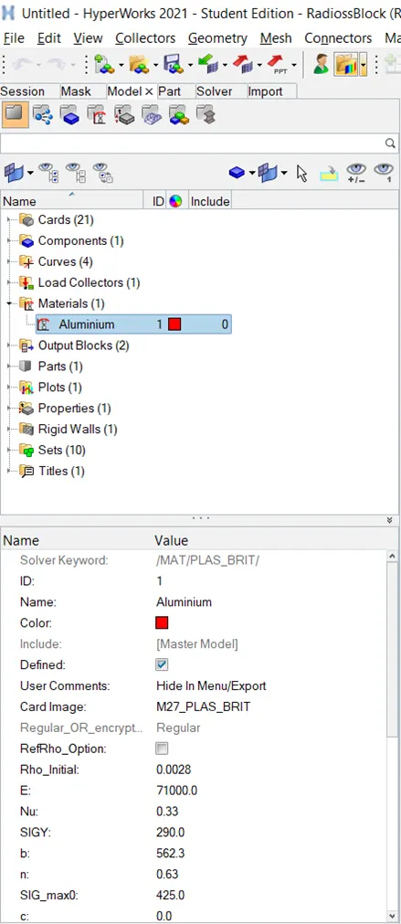
Step 3: Then run the model to separate folder with name as Law27_0000.rad. From the out put file checl the values for no of cycles, energy error, mass error and elapsed time

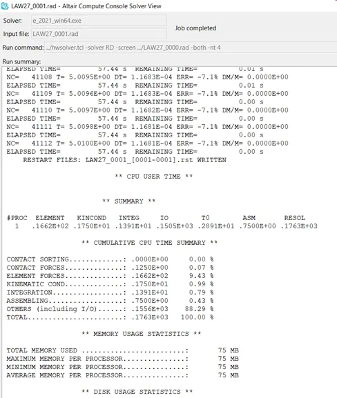
Total number of cycles = 41113

Mass error = 0
Energy error = -7.1%

Step 4 : Open the file in Hyperview and open the .h3d file and see the animation of simulation.

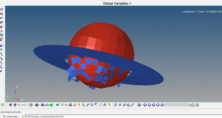
Step 5 : open the T.out file in HyperGraph 2D and take the energy graphs.

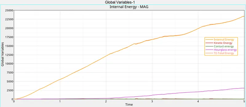
• In the case6 we are running the model by the changing shell properties I =24,I =2,I =2,N=5,I =1,I =1.
• Here we are using the law27 that means elasto-plastic materials with the brittle failure .
• Here we can observe the animation there is huge deformation taking place in between elements as shown in the above animation.
• As shown in the above graph the kinetic energy started at zero and at the time of ball hits the surface of the palte the huge deformation in occurs on the elements then they will obsorb some kinetic energy that fluctuating is shown in the above graph.

case 7:-

step 1 : Import the Law27_0000.rad in Hypermesh solver desk.

step 2 : Check the properties, Card image is M36_PLAS_TAB with same values of density, Young’s modulus, Poisson’s ratio mentioned in the video. The values are as follows EPS_p_max=0.16, EPS_t=0.1, EPS_m=0.11

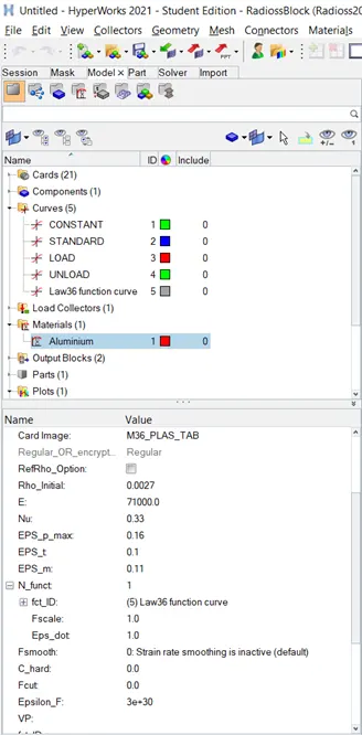
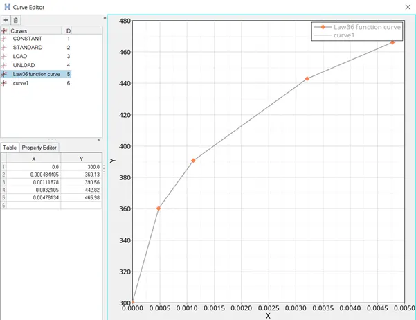
Add the curve by using given values in the video. Name the curve as Law36 Fuction curve.

Step 3: Then run the model to separate folder with name as Law36_0000.out. From the out put file check the values for no of cycles, energy error, mass error and elapsed time.

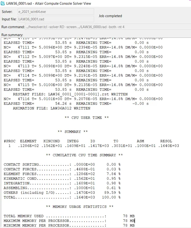
Total number of cycles= 47117

Mass error=0
Energy error= -14.8%

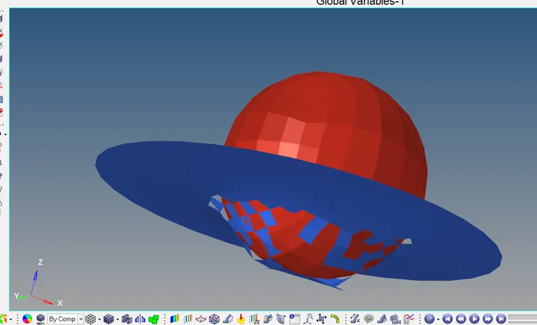
Step 4 : Open the file in Hyperview and open the .h3d file and see the animation of simulation.

Step 5 : open the T.out file in HyperGraph 2D and take the energy graphs.

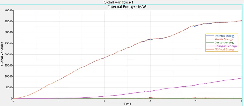
• In case7 we are using the law36 (elastic plastic piecewise linear material).This law models an isotropic elasto-plastic material using user-defined functions
• For the workhardening portion of the stress-strain curve (for example, plastic strain vs. stress) for different strain rates.
  Here we are feeding the stress strain curve to the model to interpolates the both curves For a given strain rate and For a given plastic strain.
• In order to avoid poor curve extrapolation during the strain calculation, a dummy curvedefined for a high strain rate value can be added in the model.Typically the highest strain rate curve is repeated.
• The curves have to be defined such as they don’t intersect themselves in the strain range being used.Otherwise the calculation may fail.
• Here we can observe the animation sudden deformation taking place in between elements as shown in the above animation.Here the kinetic energy and internal energy are fluctuating more compare to the previous cases as shown in the above graph

Conclusion: Did the analysis for all the given 7 cases and compared the results.