Week - 9 Material Modeling from Raw Data

AIM:

To create a material model using the data extracted from the given true stress-strain curve of graphite iron casting and validate it using the dog bone specimen.
Note: The unit system used is kg-mm-ms.

INTRODUCTION:

• To get realistic results for any analysis using FEA, a good material model for the material is necessary. A material model can have all sorts of data describing the behavior of the material in different conditions: say different tensile test curves for different strain rates and much more. This helps getting realistic behavior of the component with the material model in all sorts of situations.
• Building a material model requires test data from various experiments conducted in real life to describe the material behavior in detail. A complex analysis would benefit from a detailed material model, whereas a simpler simulation would not benefit much. The data collected from an experimental test is first cleaned to make sure any unnecessary data points are filtered out to get clear picture. Usually, the same test is repeated a number of times to ensure repeatability of the results. This test data is then inserted in the suitable format into a model: say effective stress-strain curve in x-y co-ordinates.
• A cleaner data with consistence behavior in the case of a stress strain plot, inconsistent data points should be avoided as it can affect the stability if the simulation having such a material model. A fitted curve with 98%+ accuracy can solve such issues. After matching for the unit system of the analysis, this data can be added to the simple material model to make it more detailed – for example with the use of material model such as MAT24 – linear piecewise material.
• A good practice of the material modelling procedure is the validation of the model. By performing simple analysis for which an experimental test can be performed or such data can be acquired, and then comparing the experimental and analysis results gives a good benchmark for the model. In this exercise, we try and replicate such a process.
• Material modeling is done with the help of raw data. We have to extract the data from given image. The given image gives you the Engineering Stress and Engineering Strain values. These values will produce the True stress and true strain with the help of calculations.

FOR DUCTILE MATERIAL

Stress-Strain

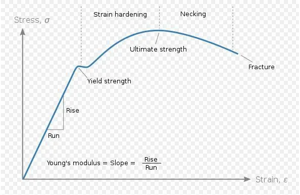
For the material the engineering stress–strain curve plot the correlation between stress and strain. It is obtained by gradually applying a load to a test coupon and measuring the deformation, from which the stress and strain can be determined eg. tensile testing. These curves provide the material properties, such as young's modulus, yield strength, and ultimate tensile strength

• The term Engineering stress is the applied load divided by the original cross-sectional area.
• The term True stress is the applied load divided by the actual cross-sectional area (changing area with respect to time)

True strain = ln(1+ engineering strain)

Effective plastic strain = total true strain - ((true stress) / (young modulus))

True stress = (engineering stress)* EXP(true strain)

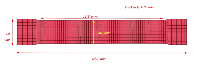
SPECIMENT CAD :

PROCEDURE :

Steps -

1. Extract the data from the diagram.
2. Clean the data and visually confirm that it matches the original data.
3. Convert the data to (kg-mm-ms) unit system
4. Process the data and create the material as demonstrated
5. Use the material model with a dog-bone specimen and validate the same.

1. Data Extraction:

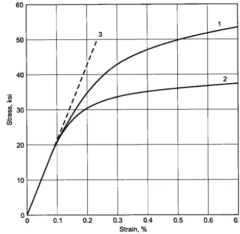
The given image file of true stress-strain graph of graphite iron casting is opened in data digitizer software to extract the data and export it as excel file.

The curve 2 is chosen to extract data of stress-strain of graphite iron casting as shown in fig.1.

Note: Ensure the data points picked is evenly spaced so as to get smooth curve and better convergence.

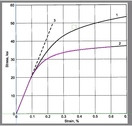
after extraction data

RAW DATA
STRAIN (in %)	STRESS(KSI)
0	0
0.03899415455	8.417084305
0.07065931743	14.96350691
0.07919104751	16.83398994
0.08772277758	18.70447297
0.09624200085	20.36698559
0.09867249127	20.78256908
0.1047424639	21.71754259
0.1120276817	22.86030785
0.1193003928	23.79510269
0.1229336216	24.21050751
0.131409071	25.14512368
0.1350360464	25.4565433
0.1471384713	26.70257908
0.1507717001	27.1179839
0.1568166591	27.63701659
0.1616526263	28.05224274
0.1664823401	28.36348368
0.1725210457	28.77853116
0.1761480211	29.08995078
0.1833894651	29.50481959
0.1906309091	29.9196884
0.1990813449	30.43836375
0.2075255273	30.8530539
0.2123489877	31.06030963
0.2207869167	31.37101457
0.2304338375	31.78552605
0.2412834967	32.19985885
0.2569503628	32.71746219
0.2665847768	32.92400325
0.278630921	33.23417218
0.288265335	33.44071325
0.3207830455	34.16378563
0.3448628271	34.57615308
0.3629164098	34.78144346
0.3942126218	35.1927389
0.4242998419	35.5002278
0.4640152226	35.91027256
0.5157579872	36.31853063
0.603601664	37.03338425
0.6565346602	37.23349324

in our case curve is fitting but if data is noisy then we use curve fitting

IF DATA SET HAVE NOISE THEN USE CURVE FITTING
EQUATION FOR CURVE FITTING
-0.843 + 300x - 965x^2 + 1394x^3 - 739x^4
	STRAIN(%)	STRESS(ksi)
	0	0
	0.03899415455	9.468866222
	0.07065931743	16.01016083
	0.07919104751	17.52581621
	0.08772277758	18.94514315
	0.09624200085	20.27053636
	0.09867249127	20.63241994
	0.1047424639	21.50567623
	0.1120276817	22.49788416
	0.1193003928	23.42992419
	0.1229336216	23.87442354
	0.131409071	24.85869132
	0.1350360464	25.25808503
	0.1471384713	26.50077325
	0.1507717001	26.84788827
	0.1568166591	27.4000852
	0.1616526263	27.8197751
	0.1664823401	28.22002248
	0.1725210457	28.69482589
	0.1761480211	28.96676392
	0.1833894651	29.48114877
	0.1906309091	29.95911749
	0.1990813449	30.47339724
	0.2075255273	30.94332337
	0.2123489877	31.19313336
	0.2207869167	31.59946025
	0.2304338375	32.01917278
	0.2412834967	32.43873344
	0.2569503628	32.95694096
	0.2665847768	33.22999551
	0.278630921	33.52860116
	0.288265335	33.73703891
	0.3207830455	34.28135216
	0.3448628271	34.56974658
	0.3629164098	34.74586077
	0.3942126218	35.00857459
	0.4242998419	35.24925366
	0.4640152226	35.59900327
	0.5157579872	36.1468091
	0.603601664	37.11840849
	0.6565346602	37.35429941

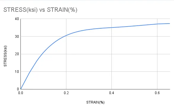
CONVERTING KSI INTO GPA

STRAIN(%)	STRESS(gpa)
0	0
0.03899415455	0.0652855345
0.07065931743	0.1103861733
0.07919104751	0.1208362492
0.08772277758	0.1306221641
0.09624200085	0.1397604286
0.09867249127	0.142255528
0.1047424639	0.1482764182
0.1120276817	0.1551174511
0.1193003928	0.1615436408
0.1229336216	0.164608356
0.131409071	0.1713946435
0.1350360464	0.1741483662
0.1471384713	0.1827163998
0.1507717001	0.1851096736
0.1568166591	0.1889169374
0.1616526263	0.1918105975
0.1664823401	0.194570206
0.1725210457	0.1978438603
0.1761480211	0.199718807
0.1833894651	0.2032653657
0.1906309091	0.206560844
0.1990813449	0.2101066781
0.2075255273	0.2133467047
0.2123489877	0.215069084
0.2207869167	0.2178706092
0.2304338375	0.2207644253
0.2412834967	0.2236571942
0.2569503628	0.2272301093
0.2665847768	0.2291127541
0.278630921	0.2311715676
0.288265335	0.2326086953
0.3207830455	0.2363616031
0.3448628271	0.2383500126
0.3629164098	0.2395642772
0.3942126218	0.2413756252
0.4242998419	0.243035049
0.4640152226	0.2454464877
0.5157579872	0.2492234759
0.603601664	0.2559224179
0.6565346602	0.2575488286

converted strain % into strain

STRAIN	STRESS(gpa)
0	0
0.0003899415455	0.0652855345
0.0007065931743	0.1103861733
0.0007919104751	0.1208362492
0.0008772277758	0.1306221641
0.0009624200085	0.1397604286
0.0009867249127	0.142255528
0.001047424639	0.1482764182
0.001120276817	0.1551174511
0.001193003928	0.1615436408
0.001229336216	0.164608356
0.00131409071	0.1713946435
0.001350360464	0.1741483662
0.001471384713	0.1827163998
0.001507717001	0.1851096736
0.001568166591	0.1889169374
0.001616526263	0.1918105975
0.001664823401	0.194570206
0.001725210457	0.1978438603
0.001761480211	0.199718807
0.001833894651	0.2032653657
0.001906309091	0.206560844
0.001990813449	0.2101066781
0.002075255273	0.2133467047
0.002123489877	0.215069084
0.002207869167	0.2178706092
0.002304338375	0.2207644253
0.002412834967	0.2236571942
0.002569503628	0.2272301093
0.002665847768	0.2291127541
0.00278630921	0.2311715676
0.00288265335	0.2326086953
0.003207830455	0.2363616031
0.003448628271	0.2383500126
0.003629164098	0.2395642772
0.003942126218	0.2413756252
0.004242998419	0.243035049
0.004640152226	0.2454464877
0.005157579872	0.2492234759
0.00603601664	0.2559224179
0.006565346602	0.2575488286

we calculate the young modulus by slope of the linear elastic region

young modulus = 141.227 GPA

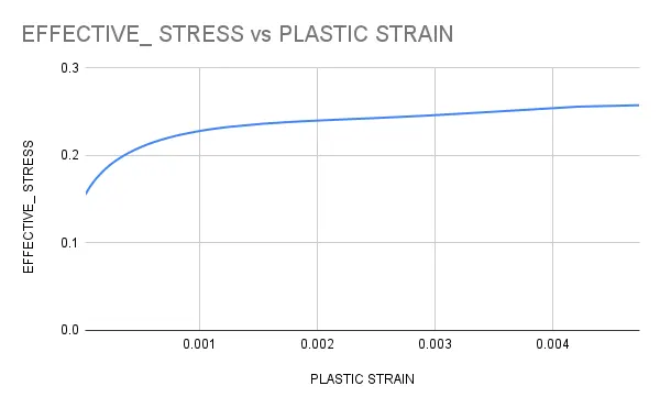
we need to define the yield limit from image it is observed that material linear elastic regioon end at about 20 ksi so our yield limit is 0.15511 GPA , from this point we define the plastic region. In LS DYNA plastic region is defined by curve between EFFEECTIVE PLASTIC STRAIN vs TRUE STRESS(correspond to the strain)

PLASTIC STRAIN	EFFECTIVE_ STRESS
0.00002192521415	0.1551174511
0.00004914992734	0.1615436408
0.00006378166046	0.164608356
0.0001004839873	0.1713946435
0.0001172552534	0.1741483662
0.0001776111921	0.1827163998
0.0001969972496	0.1851096736
0.0002304884656	0.1889169374
0.000258358785	0.1918105975
0.0002871157587	0.194570206
0.000324322809	0.1978438603
0.0003473164894	0.199718807
0.0003946185489	0.2032653657
0.0004436984518	0.206560844
0.0005030955607	0.2101066781
0.0005645954888	0.2133467047
0.0006006343143	0.215069084
0.0006651766374	0.2178706092
0.000741155388	0.2207644253
0.0008291689371	0.2236571942
0.000960538595	0.2272301093
0.001043552152	0.2291127541
0.001149435601	0.2311715676
0.001235603765	0.2326086953
0.001534207378	0.2363616031
0.001760925716	0.2383500126
0.00193286361	0.2395642772
0.002232999983	0.2413756252
0.00252212218	0.243035049
0.002902201135	0.2454464877
0.003392884782	0.2492234759
0.004223887855	0.2559224179
0.004741701572	0.2575488286

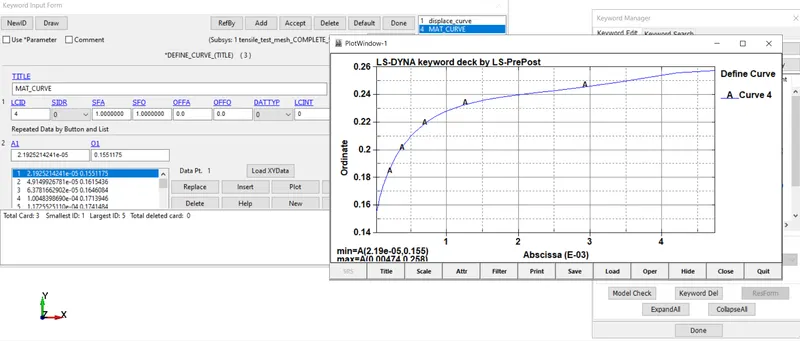
2. MATERIAL IN LS DYNA (MAT_24)

using keyword DEFINE_CURVE , apply the data (effective plastic strain vs effective stress)

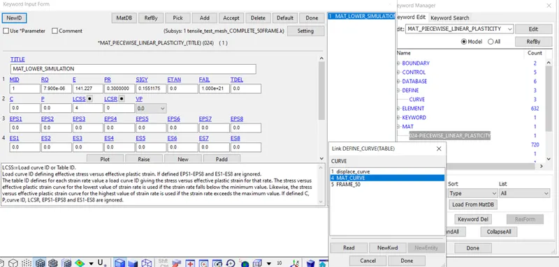
apply curve in mat 24 card

3. CASE SETUP

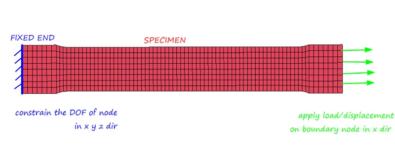
defining the other card

• SECTION_SHELL
• BOUNDARY_PRESCRIBED_MOTION_SET
• BOUNDARY_SPC
• CONTROL_TERMINATION
• CONTROL_IMPLICIT_GENERAL
• CONTROL_IMPLICIT_AUTO
• CONTROL_IMPLICIT_SOLVER
• CONTROL_IMPLICIT_SOLUTION
• DATABASE_ACII(glstat,matsum,eleout)
• DATABASE_D3PLOT, DATABASE_EXTENT_BINARY

we can setup the deck

RESULT :

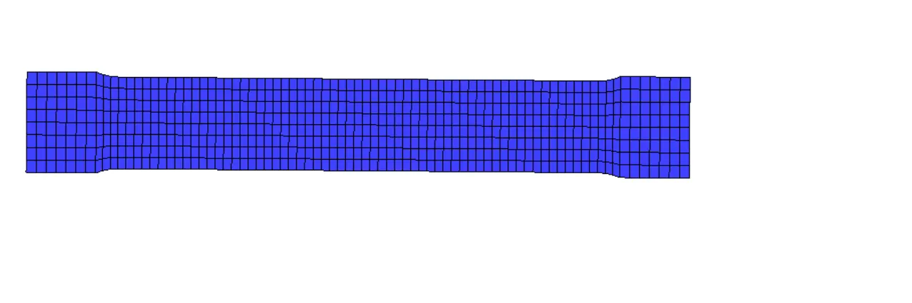
after running the simualtion we acn get the Von misses stress and x dir strain

X DIRECTION STRAIN	VON MISSES STRESS
0.00E+00	0.00E+00
1.43E-04	2.07E-02
2.87E-04	4.13E-02
4.30E-04	6.20E-02
5.73E-04	8.26E-02
7.16E-04	1.03E-01
8.60E-04	1.24E-01
1.00E-03	1.44E-01
1.15E-03	1.60E-01
1.30E-03	1.73E-01
1.45E-03	1.85E-01
1.60E-03	1.94E-01
1.75E-03	2.02E-01
1.91E-03	2.08E-01
2.06E-03	2.14E-01
2.22E-03	2.20E-01
2.38E-03	2.24E-01
2.53E-03	2.28E-01
2.69E-03	2.31E-01
2.87E-03	2.33E-01
3.06E-03	2.35E-01
3.20E-03	2.37E-01
3.42E-03	2.38E-01
3.66E-03	2.40E-01
3.85E-03	2.41E-01
3.88E-03	2.41E-01
3.92E-03	2.41E-01
4.34E-03	2.44E-01
4.45E-03	2.44E-01
4.58E-03	2.45E-01
4.73E-03	2.46E-01
4.86E-03	2.47E-01
5.02E-03	2.48E-01
5.17E-03	2.50E-01
5.33E-03	2.51E-01
5.46E-03	2.52E-01
5.62E-03	2.53E-01
5.76E-03	2.54E-01
5.91E-03	2.55E-01
6.01E-03	2.56E-01
6.42E-03	2.57E-01
6.47E-03	2.57E-01

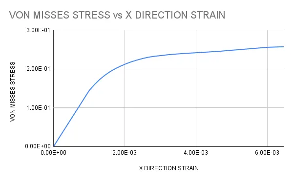
COMPARISION BETWEEN RAW DATA AND SIMULATED DATA

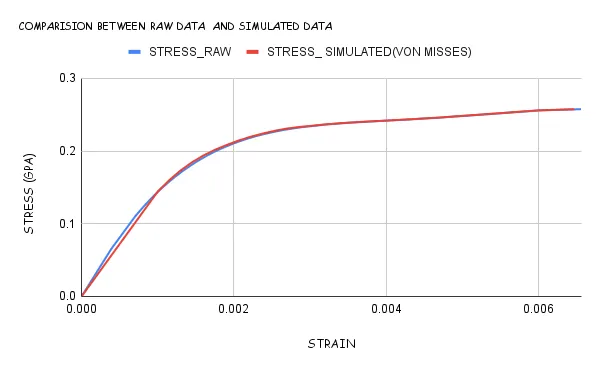
from above graph it is observed that we successfully model the material model