FVM Literature Review

Finite Difference method:

• In simple terms, the main objective of FDM is to convert the partial differential equations into algebraic equations, such as; `(deltau)/(deltax) = (U^(i+1)-U^(i-1))/(2.Deltax)`
• The major disadvantage of FDM is the mapping process. The mapping of complex geometry or non-aligned f=grids is time-consuming and needs complex coding.
• Obtaining the finite difference equations from the differential terms is done with the help of Taylor's theorem/Taylor series expansions.
• One of the advantages of FDM is straight forward geometries are solved using simple codes with a minimal computational cost.

Finite Element Method:

• Foremost, an element is a non-physical imaginary part of the body having a mathematical nature. A body/part is considered to be divided into a large number of smaller elements having grid points.
• Each element is governed by a simple algebraic equation which is later assembled/integrated to model the entire domain.
• Unlike FDM, FEM can handle irregular-shaped bodies, large deformations, non-linear behavior & non-linear material properties efficiently.
• But, although having so many advantages in FEM, the drawback in FEM is, the equations are not conserved which leads to errors in stability and continuity.

Finite Volume Method:

• FVM is a volume-based method where the domain is split into smaller sections of equal volume grids & the properties of the volume are taken as the average of the small volume grids & integrated to find the solution of the entires domain.
• Unlike Element, Volume is a physical quantity leading to physical interpretations of the domain.
• Some of the advantages of FVM are,
  • It can handle curved boundaries with ease.
  • The governing equations are directly integrated leading to simple coding and lesser computational time.
• Furthermore, the process of FVM can be explained with the help of a 1-D steady-state heat conduction equation.

Consider an example of a 1-D heat conduction problem in a rod. Therefore, 1-D steady-state diffusion of property 'ϕ' with a source term 'S' and diffusion coefficient 'Γ' are considered as in the domain shown below.

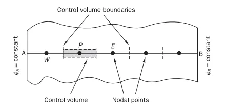
The process is governed by the following equation, `d/(dx)(Gamma(dphi)/(dx))+S=0`.

The boundary values of 'ϕ' at A & B are considered to be constant, that is, ϕA = constant & ϕB = constant.

The FVM process to solve for the 1-D steady-state heat conduction equation goes through the following steps:

1. Grid generation
2. Discretization
3. Solution of equations

Step 1: Grid generation:

The domain is discretized into a smaller number of control volumes as shown in the above figure.

Each node as shown in the above figure is surrounded by a control volume as the boundaries of the cell are considered to be at the mid-way between the two adjacent nodes. The domain is simplified by giving notations to each cell for easy understanding as shown in the below figure.

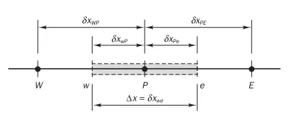
Simple notations are used for the process. The distances between the nodes and the boundaries of the cell are also shown in the figure.

Step 2: Discretization

In this step, the key role is to integrate the governing equations over a control volume to yield a discretized equation at its nodal point P. For the above control volume, the governing equation is converted as,

With the help of the central differencing scheme, for a uniform grid linearly interpolated values for 'Γw' & 'Γe' can be given as, `Gamma^w = (Gamma^W+Gamma^P)/2`, `Gammae = (Gamma^P+Gamma^E)/2`. Therefore the diffusion terms can be written as,

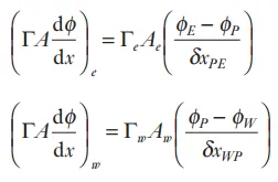
When it comes to the source term, it is a bit different from the diffusive flux terms. In practical cases, the source term may be a function of the dependent variable. Therefore, in cases as those, the FVM approximates the source term as a linear form which is represented as,

`barSDeltaV=S^u+S^p phi^P`

Therefore, the discretized equation can be rearranged as

The above equation is set up for each nodal point and the set of equations obtained for all nodes are then solved to obtain the diffusion of the property 'ϕ'.

Gradient Schemes:

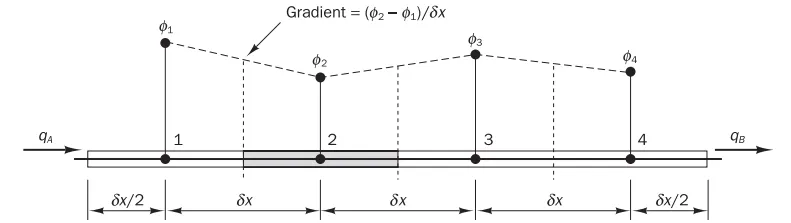
This scheme can be simply explained with the help of the below diagram.

If we want to find the temperature gradient at nodal point P, we use the values at the neighboring nodes w & e to determine the temperature at P. This scheme is generally known as a gradient scheme.

There are some cases, where the central differencing scheme fails to interpret the values, such as in problems involving convection & diffusion at the same time. This issue leads to exploring the properties of the discretization schemes. The most important properties to be considered are

1. Conservativeness
2. Boundedness
3. Transportiveness

Interpolation Schemes:

In FVM, we are considering the values to be stored in the center of the control volume. But, it is important to interpolate the cell center results to the face centers, which helps in obtaining the flux values for the surface integral in the governing equation. Therefore, the values at other than the computational nodes are required which are unknown. So, with the help of some mathematical approximations/schemes, the unknown values are computed.

There are various types of interpolation schemes such as:

1. Central differencing scheme
2. Upwind differencing scheme
3. Hybrid differencing scheme
4. Quadratic upwind differencing (QUICK) scheme
5. Total variation diminishing (TVD) scheme

1. Central differencing scheme

Although the truncation error of the CDS is second-order, CDS uses consistent expressions to estimate convective and diffusive fluxes at the cell faces. CDS uses linear interpolation to evaluate the unknown cell face values. One of the disadvantages of CDS is its inability to determine the flow direction.

2. Upwind differencing scheme

Upwind differencing, also known as donor cell differencing takes into account the flow direction when estimating the cell face value. Therefore, the value of 'ϕ' at the cell face is considered to be equal to the value at the upstream node.

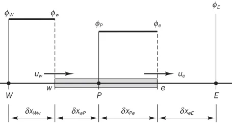
In the above figure, the rate of convection is higher than the diffusion, which prevents the use of Central differencing scheme. Therefore, when the flow direction is from west to east, the cell face value is considered to be equal to the upwind node, i.e., `phi^w = phi^W; phi^e = phi^P`which brings a change in the discretised equation.

3. Hyrbid differencing scheme

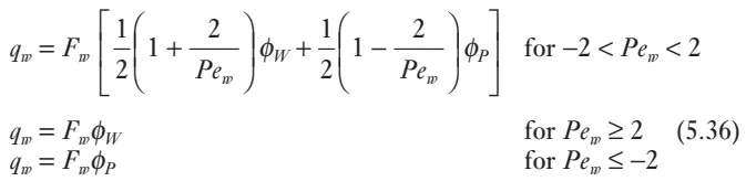
This scheme is a combination of central and upwind differencing scheme. The central differencing scheme which is a second-order accurate and upwind differencing scheme a first-order accurate is combined to evaluate the net flux through each control volume face. As mentioned earlier, the properties of the schemes are to monitored carefully to evaluate the discretized equations properly. Therefore, the peclet number which determines the transportiveness property of a fluid flow is calculated at each face of the control volume. The below equation shows the peclet number for a west face,

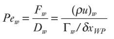
Therefore, the hybrid differencing formulae for the net flux per unit area through the west face can be written as,

4.Quadratic upwind differencing (QUICK) scheme

The errors that occurred in the first-order accuracy schemes such as hybrid and upwind can be minimised by employing higher-order disretization which involves more neighbor points reducing the discretization erros. Althought the earlier schemes are stable and obey the transportiveness property, the first-order accuracy makes them liable to numerical diffusion errors.

The quadratic upstream interpolation for convective kinetics (QUICK) scheme uses a three-point upstream-weighted quadratic interpolation to evaluate the cell face values. The below figure shows the quadratic profiles used in QUICK scheme.

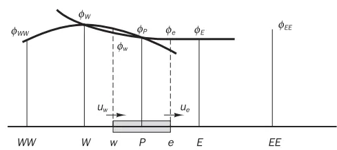
As shown in the above figure to evaluate 'ϕw' a quadratic fit through WW, W & P is used.

5. Total variation diminishing (TVD) schemes

These third-order and above schemes are specially formulated to achieve oscillation-free/ minimal truncation error solutions. The problems such as undershoots and overshoots in the QUICK scheme and other higher-order schemes can be avoided using this scheme.

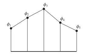
TVD is a monotonicity preserving scheme, which means it does not create new undershoots and overshoots in the solution. An example of a discrete data set is shown in the below image to illustrate the total variation.

Flux limiters:

Flux limiters are used in higher-order schemes to make the solution oscillation-free or total variation diminishing. The flux limiters can be generally referred to as limiters on system fluxes. So generally, these schemes are used to limit the spatial derivatives to realistic values.

The flux limiter functions were originally introduced to make the above schemes higher-order as the low-order schemes are reckless under discontinuity or shocks even though they are usually stable. On the other hand, the higher-order schemes are less stable and show osciallations in the regions of discontinuity. Therefore, high resolution schemes were introduced which show greater efficiency and accuracy in the presence of shocks and discontinuity. These limiter functions work well with high resolution schemes to avoid the wiggles in the solution.

Some of themost frequently used limiter functions are shown in the below table.

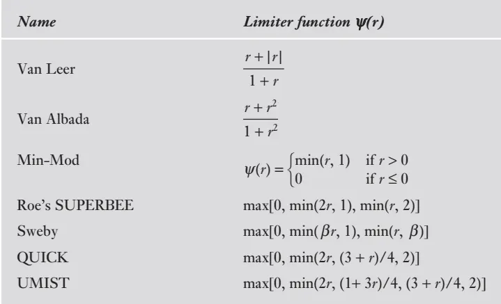
These above limiter functions give second-order accurate solutions that are free from non-physical wiggles.