Simulation of Flow through a pipe in OpenFoam
Aim:-
To simulate an axisymmetric laminar flow through a cylindrical pipe applying the wedge boundary condition using OpenFlow and MATLAB.
Objectives:-
- To perform simulation of a laminar flow through a constant cross-section pipe whose Reynolds number is 2100 at the inlet.
- Validate the results with the Hagen- Poiseuille's equations for the fully developed flow.
- Obtain blockMeshdict file with the help of MATLAB code.
- Post-process the model to obtain numerical results to validate with hydro-dynamic length.
- Examine the numerical results for velocity and shear stress and validate with analytical results.
Laminar Flow:-
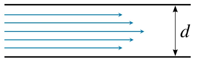
A fluid flow in a closed cylindrical pipe that has streamlines parallel to each other along the length of the cylinder is called a laminar flow. In a laminar flow, the fluid properties such as pressure, velocity, etc are considered constant with respect to time.
Axi-Symmetric Flow:-
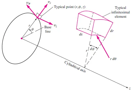
The flow pattern which is identical in every plane that passes through a certain straight line is called an axisymmetric flow. In an axisymmetric flow, the symmetry is rotatory.
Hydrodynamic Entrance Length:-
When a fluid flows in a cylindrical pipe, the advection between the fluid and the internal surfaces of the cylindrical pipe creates friction and disrupts the flow. Due to the boundary thickness concept, the flow will not be fully developed at the entrance of the pipe flow. The fluid travels a certain distance inside the pipe before it reaches a fully developed state. This concept is called the hydrodynamic entrance length.
The region from the fluid flow entrance to the fully developed flow point is called the hydrodynamic entrance region. The flow will be inviscid and irrotational in the hydrodynamic entrance region. The length of the hydrodynamic region along the pipe can be described with the help of the dimensionless number, known as the Entrance length Number.
The Entrance length can be mathematically expressed as,

Reynolds number `Re = (rhoVD)/mu`
Hagen-Pousielles Equation:-
Fluid flows from a high-pressure point to a low-pressure point due to the pressure difference. This pressure drop is the key point to determine the velocity of the fluid. Therefore, the pressure gradient (dp/dx), the difference in pressure along the length of the pipe is the major factor to determine the flow of the fluid.
It can be concluded that fluid flow is dependant on factors such as pressure gradient. Similarly, the Hagen-Pousielle equation is used to determine this pressure drop in a cylindrical pipe laminar flow, which depends on factors such as Flow rate, Dynamic viscosity, length, and radius of the pipe. The equation can be represented mathematically as,
`DeltaP=(8muLQ)/(piR^4)`
`DeltaP` Pressure Difference
`mu` Dynamic Viscosity
`Q` Volumetric flow rate = Area `A` `.` Velocity of Fluid `V`
`L` Length of Pipe
`R` Radius of Pipe = Half of Diameter `D/2`
`A` Area = `pi.R^2`
Therefore, considering the above parameters, the Hagen-Pousielle equation can be rewritten as,
`DeltaP=(32muLV)/D^2`
Assumptions:-
Water Properties at 25°C:
- Dynamic Viscosity `mu` = 8.9e-4 `Pa.s`
- Density `rho` = 997 `(kg)/m^3`
Reynolds Number `Re` = 2100 (Laminar)
Diameter of Pipe `D` = 0.02 `m`
Wedge angle `theta` = 3°
Entry length calculations:
- Entrance Length `Le = 0.05.Re.D` = 2.1 `m`
- Total length of pipe `Lt = 0.9+Le` = 3.0 `m`
Velocity Calculations:
- Average velocity `Vavg = (Re.mu)/(rho.D)` = 0.0937 `m/s`
- Maximum velocity `Vmax = 2*Vavg` = 0.1874 `m/s`
Shear stress `tau = mu(du)/(dy)` Pa
- `u` - velocity
Workflow:-
- Write a Matlab code to generate a blockmeshdict file.
- Run the blockmeshdict file to generate a section of the pipe along the length.
- Edit the controldict, pressure, and velocity file.
- Run the icoFoam command.
- Validate the output shear stress values from icoFoam by comparing them with analytical solutions
- Validate Hydro-dynamic length with the numerical result
- Validate the fully developed flow velocity profile with its analytical profile
- Validate maximum velocity and pressure drop for fully developed flow
Pre-Processing:-
- Matlab code is written to generate a blockmeshdict file. The 'fopen' command is used to create a new file and input data in it. The Matlab code is run to get an output blockmeshdict file.
Matlab Code:-
%Simulation of flow through pipe
clear all
close all
clc

%Water @ 25°C
D = 0.02; %Diameter of pipe meters
r = D/2; %Radius meters
Re = 2100; %Reynolds no
mu = 8.90e-4; %Dynamic Viscocity kg/m.s
rho = 997.13; %Density kg/m^3
nu = 8.935e-7; %Kinemcatic Viscocity m^2/s
Le = Re*0.05*D; %Hydrodynamic entrance length for laminar flow meters
Lt = 0.9 + Le; %Total length meters
theta = 3; % Wedge Angle Degrees
Vavg = (Re*mu)/(rho*D); %Average Velocity m/s
Vmax = 2*Vavg; %Maximum velocity m/s
dP = (32*mu*Le*Vavg)/(D^2); %Pressure drop equation Pa
kine_p = dP/rho; %Kinematic Pressure

%blockMesh dict
%Vertices
v0 = [0 0 0];
v1 = [0 r*cosd(theta/2) -r*sind(theta/2)];
v2 = [0 r*cosd(theta/2) r*sind(theta/2)];
v3 = [Lt 0 0];
v4 = [Lt r*cosd(theta/2) -r*sind(theta/2)];
v5 = [Lt r*cosd(theta/2) r*sind(theta/2)];
%Grading
g1 = 50;
g2 = 1;
g3 = 200;
%creating and opening blockMesh dict file
bM = fopen('blockMeshDict','w');
%Header files
fprintf(bM, '%sn', '/*--------------------------------*- C++ -*----------------------------------*');
fprintf(bM, '%sn', ' =========                 |                                                   ');
fprintf(bM, '%sn', ' \      /  F ield         | OpenFOAM: The Open Source CFD Toolbox             ');
fprintf(bM, '%sn', '  \    /   O peration     | Website:  https://openfoam.org                    ');
fprintf(bM, '%sn', '   \  /    A nd           | Version:  7                                       ');
fprintf(bM, '%sn', '    \/     M anipulation  |                                                   ');
fprintf(bM, '%sn', '*---------------------------------------------------------------------------*/');
fprintf(bM,'%sn','FoamFile'); %Dictionary
fprintf(bM,'%sn','{');
fprintf(bM,'%sn','    version     2.0;');
fprintf(bM,'%sn','    format      ascii;');
fprintf(bM,'%sn','    class       dictionary;');
fprintf(bM,'%sn','    object      blockMeshDict;');
fprintf(bM,'%sn','}');
fprintf(bM,'%snn','// * * * * * * * * * * * * * * * * * * * * * * * * * * * * * * * * * * * * * //');
fprintf(bM,'%snn','convertToMeters 1;');

%Defining Vertices
fprintf(bM,'%sn','vertices');
fprintf(bM,'%sn','(');
fprintf(bM,'t(%d %d %d)n',v0(1),v0(2),v0(3));
fprintf(bM,'t(%d %d %d)n',v1(1),v1(2),v1(3));
fprintf(bM,'t(%d %d %d)n',v2(1),v2(2),v2(3));
fprintf(bM,'t(%d %d %d)n',v3(1),v3(2),v3(3));
fprintf(bM,'t(%d %d %d)n',v4(1),v4(2),v4(3));
fprintf(bM,'t(%d %d %d)n',v5(1),v5(2),v5(3));
fprintf(bM,'%snn',');');

% Defining Blocks
fprintf(bM,'%sn','blocks');
fprintf(bM,'%sn','(');
fprintf(bM,'thex (0 1 2 0 3 4 5 3) (%d %d %d) %s (%d 1 1)n',g1,g2,g3,'simpleGrading',0.2);
fprintf(bM,'%snn',');');

% Defining Edges
fprintf(bM,'%sn','edges');
fprintf(bM,'%sn','(');
fprintf(bM,'tarc %d %d (%d %d %d)n',1,2,0,r,0);
fprintf(bM,'tarc %d %d (%d %d %d)n',4,5,Lt,r,0);
fprintf(bM,'%sn',');');

% Defining Boundaries
fprintf(bM,'%sn','boundary');
fprintf(bM,'%sn','(');
fprintf(bM,'tinletnt{n');
fprintf(bM,'tttype patch;n');
fprintf(bM,'tt faces ntt(n');
fprintf(bM,'ttt(0 1 2 0)n');
fprintf(bM,'tt);nt}n');

fprintf(bM,'toutletnt{n');
fprintf(bM,'tttype patch;n');
fprintf(bM,'tt faces ntt(n');
fprintf(bM,'ttt(3 4 5 3)n');
fprintf(bM,'tt);nt}n');

fprintf(bM,'tfrontnt{n');
fprintf(bM,'tttype wedge;n');
fprintf(bM,'tt faces ntt(n');
fprintf(bM,'ttt(0 3 5 2)n');
fprintf(bM,'tt);nt}n');

fprintf(bM,'tbacknt{n');
fprintf(bM,'tttype wedge;n');
fprintf(bM,'tt faces ntt(n');
fprintf(bM,'ttt(0 3 4 1)n');
fprintf(bM,'tt);nt}n');

fprintf(bM,'ttopnt{n');
fprintf(bM,'tttype wall;n');
fprintf(bM,'tt faces ntt(n');
fprintf(bM,'ttt(1 2 5 4)n');
fprintf(bM,'tt);nt}n');

fprintf(bM,'taxisnt{n');
fprintf(bM,'tttype empty;n');
fprintf(bM,'tt faces ntt(n');
fprintf(bM,'ttt(0 3 3 0)n');
fprintf(bM,'tt);nt}n');
fprintf(bM,');nn');
fprintf(bM,'mergePatchPairsn(n);nn');
fprintf(bM,'// ************************************************************************* //');
fclose(bM);
Blockmeshdict File:-
- Blockmeshdict file is a dictionary file used to create geometrical meshed models of 1 or more three-dimensional, hexahedral blocks with grading and curved edges.
- The geometry is specified by vertices, blocks, edges (straight lines, arcs, or splines), and boundaries.
- The 'blockMesh' command is used to read the blockmeshdict file and generate the meshed model into points, faces, and cells.
/*--------------------------------*- C++ -*----------------------------------*
 =========                 |
 \      /  F ield         | OpenFOAM: The Open Source CFD Toolbox
  \    /   O peration     | Website:  https://openfoam.org
   \  /    A nd           | Version:  7
    \/     M anipulation  |
*---------------------------------------------------------------------------*/
FoamFile
{
    version     2.0;
    format      ascii;
    class       dictionary;
    object      blockMeshDict;
}
// * * * * * * * * * * * * * * * * * * * * * * * * * * * * * * * * * * * * * //

convertToMeters 1;

vertices
(
	(0 0 0)
	(0 9.996573e-03 -2.617695e-04)
	(0 9.996573e-03 2.617695e-04)
	(3 0 0)
	(3 9.996573e-03 -2.617695e-04)
	(3 9.996573e-03 2.617695e-04)
);

blocks
(
	hex (0 1 2 0 3 4 5 3) (50 1 200) simpleGrading (2.000000e-01 1 1)
);

edges
(
	arc 1 2 (0 1.000000e-02 0)
	arc 4 5 (3 1.000000e-02 0)
);
boundary
(
	inlet
	{
		type patch;
		 faces
		(
			(0 1 2 0)
		);
	}
	outlet
	{
		type patch;
		 faces
		(
			(3 4 5 3)
		);
	}
	front
	{
		type wedge;
		 faces
		(
			(0 3 5 2)
		);
	}
	back
	{
		type wedge;
		 faces
		(
			(0 3 4 1)
		);
	}
	top
	{
		type wall;
		 faces
		(
			(1 2 5 4)
		);
	}
	axis
	{
		type empty;
		 faces
		(
			(0 3 3 0)
		);
	}
);

mergePatchPairs
(
);

// ************************************************************************* //
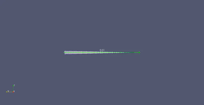
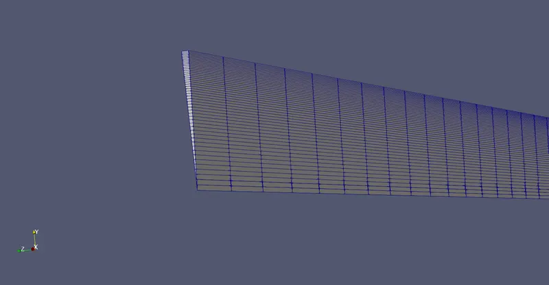
Meshed Model:
Controldict File:-
- The controldict file is another dictionary file that majorly impacts the start and end of the simulation.
- Main parameters for a simulation such as a start time, end time, time step are represented under the controldict file.
/*--------------------------------*- C++ -*----------------------------------*
  =========                 |
  \      /  F ield         | OpenFOAM: The Open Source CFD Toolbox
   \    /   O peration     | Website:  https://openfoam.org
    \  /    A nd           | Version:  7
     \/     M anipulation  |
*---------------------------------------------------------------------------*/
FoamFile
{
    version     2.0;
    format      ascii;
    class       dictionary;
    location    "system";
    object      controlDict;
}
// * * * * * * * * * * * * * * * * * * * * * * * * * * * * * * * * * * * * * //

application     icoFoam;

startFrom       startTime;

startTime       0;

stopAt          endTime;

endTime         50;

deltaT          0.01;

writeControl    timeStep;

writeInterval   200;

purgeWrite      0;

writeFormat     ascii;

writePrecision  6;

writeCompression off;

timeFormat      general;

timePrecision   6;

runTimeModifiable true;


// ************************************************************************* //
- The input boundary conditions in OpenFOAM are given using the initial conditions file such as p and u file.
- The p file is used to give the pressure boundary conditions and u file is used to give the velocity boundary conditions at the initial stage of the simulation.
- The p and u file themselves are other dictionary files.
Pressure 'p' File:-
/*--------------------------------*- C++ -*----------------------------------*
  =========                 |
  \      /  F ield         | OpenFOAM: The Open Source CFD Toolbox
   \    /   O peration     | Website:  https://openfoam.org
    \  /    A nd           | Version:  7
     \/     M anipulation  |
*---------------------------------------------------------------------------*/
FoamFile
{
    version     2.0;
    format      ascii;
    class       volScalarField;
    object      p;
}
// * * * * * * * * * * * * * * * * * * * * * * * * * * * * * * * * * * * * * //

dimensions      [0 2 -2 0 0 0 0];

internalField   uniform 0;

boundaryField
{
    outlet
    {
        type            fixedValue;
        value           uniform 0.018;
    }

    inlet
    {
        type            zeroGradient;
    }

    front
    {
        type            wedge;
    }

    back
    {
        type            wedge;
    }

    top
    {
        type            zeroGradient;
    }
}

// ************************************************************************* //
Velocity 'U' File:-
/*--------------------------------*- C++ -*----------------------------------*
  =========                 |
  \      /  F ield         | OpenFOAM: The Open Source CFD Toolbox
   \    /   O peration     | Website:  https://openfoam.org
    \  /    A nd           | Version:  7
     \/     M anipulation  |
*---------------------------------------------------------------------------*/
FoamFile
{
    version     2.0;
    format      ascii;
    class       volVectorField;
    object      U;
}
// * * * * * * * * * * * * * * * * * * * * * * * * * * * * * * * * * * * * * //

dimensions      [0 1 -1 0 0 0 0];

internalField   uniform (0 0 0);

boundaryField
{
    inlet
    {
        type            fixedValue;
        value           uniform (0.093718973453812 0 0);
    }

    outlet
    {
        type            zeroGradient;
    }

    front
    {
        type            wedge;
    }

    back
    {
        type            wedge;
    }

    top
    {
        type            noSlip;
    }
}

// ************************************************************************* //
Transport Properties File:-
- transportProperties file is another dictionary file used to include the constant properties such as Viscosity `mu`, Strain rate `dotgamma`etc., used in the models such as Newtonian model, Power Law model, etc.
/*--------------------------------*- C++ -*----------------------------------*
  =========                 |
  \      /  F ield         | OpenFOAM: The Open Source CFD Toolbox
   \    /   O peration     | Website:  https://openfoam.org
    \  /    A nd           | Version:  7
     \/     M anipulation  |
*---------------------------------------------------------------------------*/
FoamFile
{
    version     2.0;
    format      ascii;
    class       dictionary;
    location    "constant";
    object      transportProperties;
}
// * * * * * * * * * * * * * * * * * * * * * * * * * * * * * * * * * * * * * //

nu              [0 2 -1 0 0 0 0] 8.935e-7;


// ************************************************************************* //
Post-Processing:-
Results:-
- A foam file is created after the end of the simulation for post-processing.
- Paraview is used for the post-processing of the pipe flow.
- The velocity profiles at different lengths are plotted to observe the variations in the pipe flow.
Pressure Contour:
Pressure Plot:
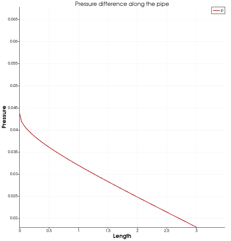
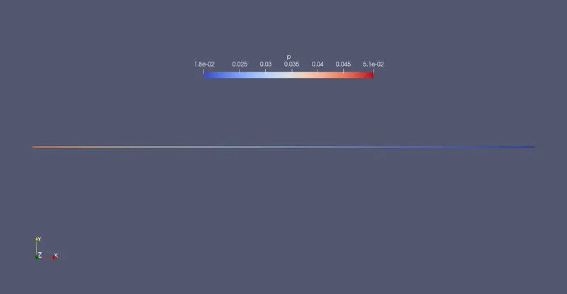
- The major factor for fluid flow is the pressure difference or the pressure drop in the fluid. Fluid flows from high-pressure point to low-pressure point which creates a pressure drop. This pressure drop can be clearly observed in the contour as well as the plot. The maximum pressure at the entrance of the pipe is found to be 0.043 Pa.
- The pressure drop can be simply calculated as the difference between the pressure points at the entrance of the pipe and the end of the pipe. `DeltaP = P1 - P2 = 0.043 - 0.018 = 0.025 Pa`
Velocity Contour:
1. Velocity contour plot at the entrance of the pipe.
2. Velocity contour plot at the end of the plot.
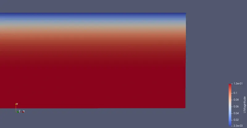
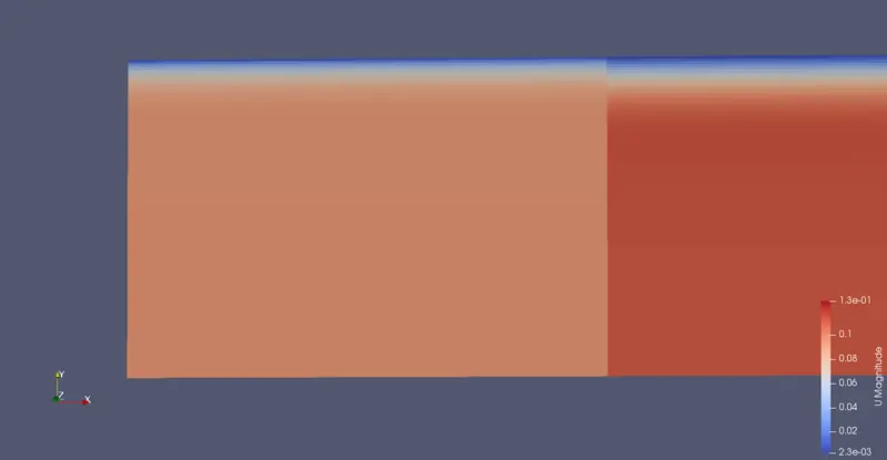
- The contour clearly depicts that the velocity at the top of the pipe is almost equal to zero and the pipe's radius is maximum. Therefore, it can be concluded that the results match with the theoretical concepts that, due to the boundary layer, the velocity of the flow is very less and the radius of the pipe the velocity reaches maximum.
- It can also be observed that at the entrance of the pipe, the velocity is almost constant, but due to the o slip boundary condition, the velocity profile change along the pipe is entirely different when velocity at entrance and velocity at the end of the pipe are compared.
Velocity Profile Plots:
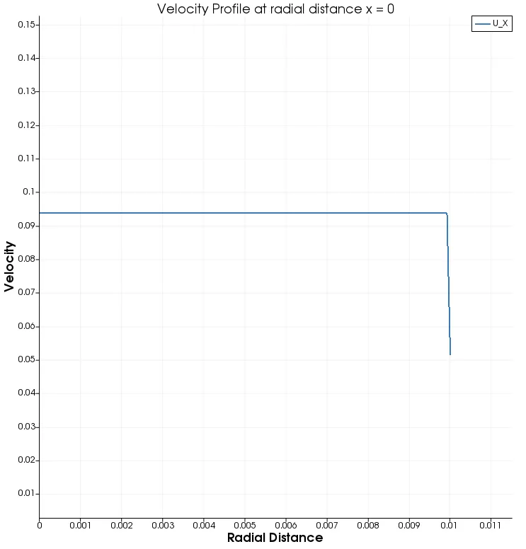
1. Velocity at radial distance x = 0m from the entrance of the pipe.
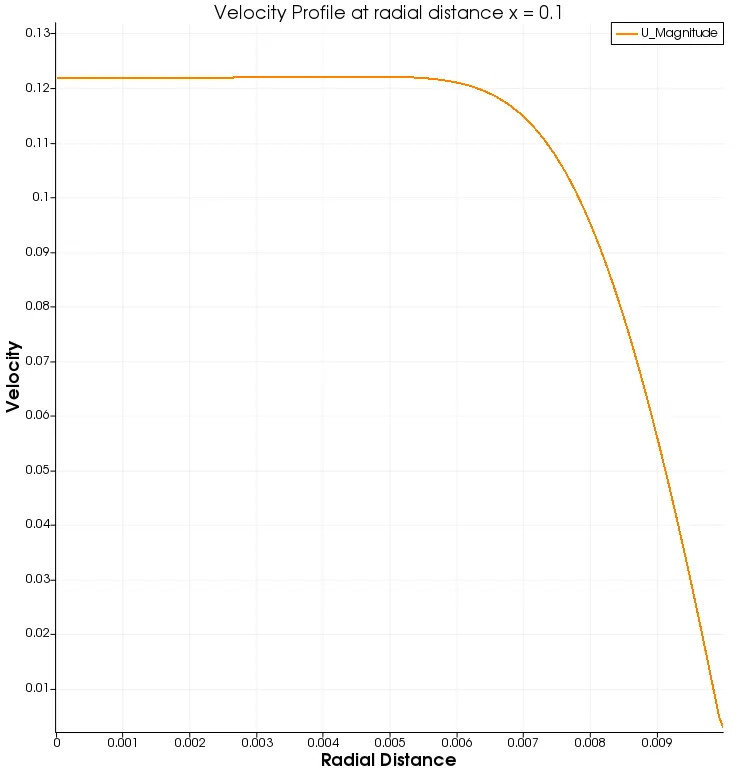
2. Velocity at radial distance x = 0.1m from the entrance of the pipe.
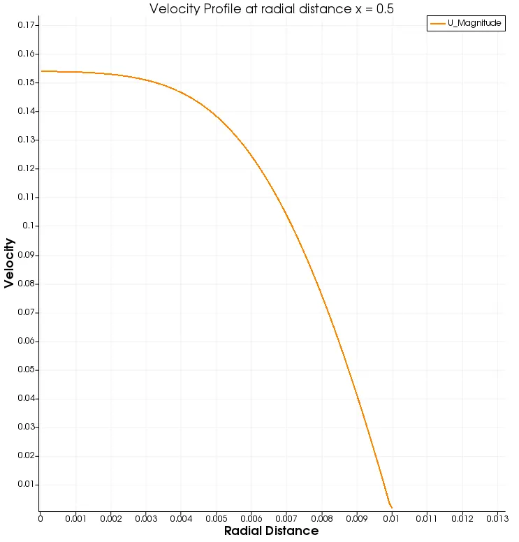
3. Velocity at radial distance x = 0.5m from the entrance of the pipe.
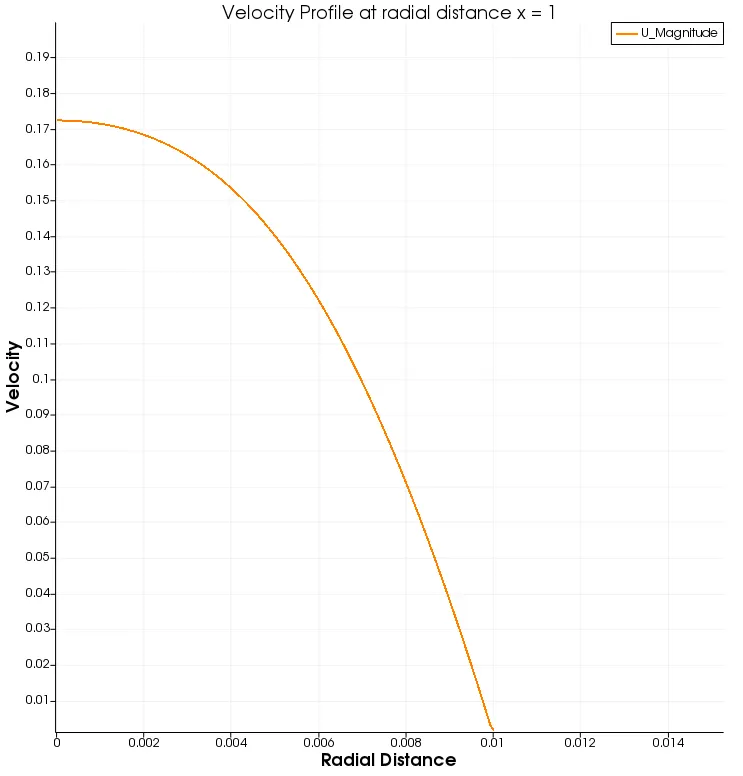
4. Velocity at radial distance x = 1m from the entrance of the pipe.
5. Velocity at radial distance x = 1.5m from the entrance of the pipe.
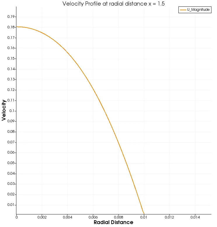
6. Velocity at radial distance x = 2m from the entrance of the pipe.
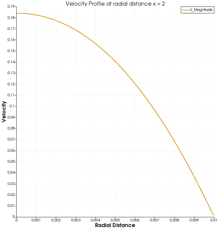
7. Velocity at radial distance x = 2.1m from the entrance of the pipe.
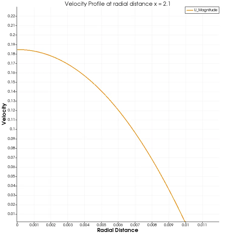
8. Velocity at radial distance x = 2.5m from the entrance of the pipe.
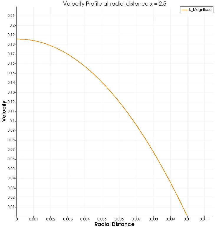
9. Velocity at radial distance x = 3m from the entrance of the pipe.
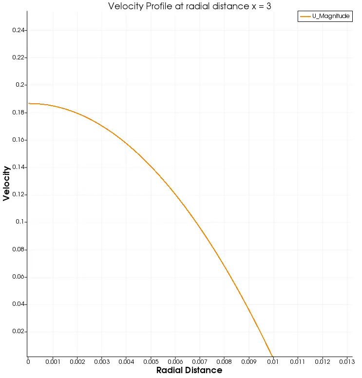
- From the above plots, it can be observed that the average velocity of the flow at the entrance of the pipe is at a constant value. But a slight difference in the x-direction is when the plot is recorded at x =0.1m, the velocity curve changes. This change in the velocity profile is due to the boundary layer concept. Due to the boundary layer thickness, the velocity curve along the radial distance varies. This variation in the velocity profile carries on until the flow reaches the hydrodynamic length.
- As it can be observed, the velocity profile at radial distance x = 2.1 from the entrance of the length, which technically speaking is the point where the flow converts from hydrodynamic to fully developed. It can also be observed that the velocity profile remains the same from 2.1m to 3m. This clearly implies that the flow is fully developed and will remain the same along the pipe from 2.1m.
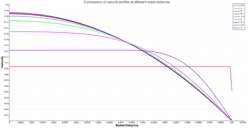
- All the velocity profiles in a single plot show the variation in the velocity along with the radial distance at different lengths. The plot depicts that the velocity profile variation from x = 2.1m to 3m is minimal. This variation in the velocity will also result in the difference in the shear stress and the flow as the flow velocity is directly proportional to the shear stress. At the wall, the velocity is less and at the pipe axis, the velocity is maximum.
Shear stress plot:
- To obtain the shear stress plot in ParaView, du/dy which is called the velocity gradient must be calculated. This can be done with the help of the calculator and gradient of unstructured data set command. The velocity gradient is then again multiplied with the constant value of dynamic viscosity using the calculator command at each mesh point in the geometry.
- Using the plot over line command, the shear stress along the pipe from the entrance of the pipe to the end of the pipe is obtained.
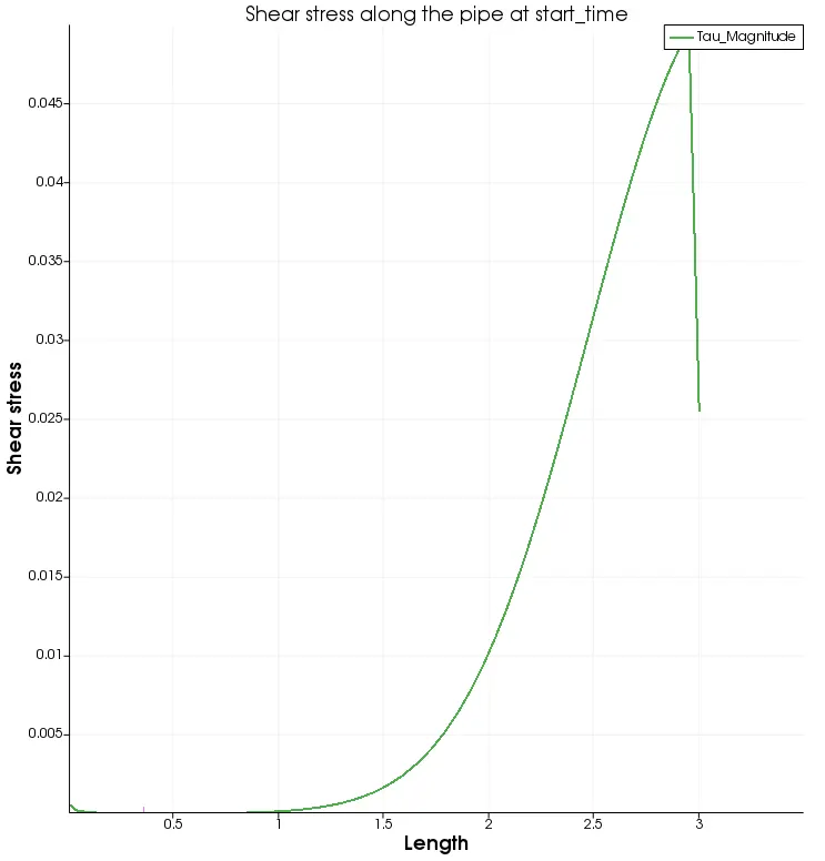
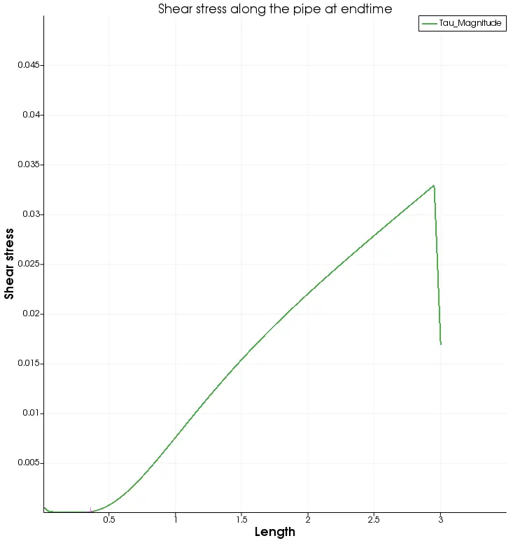
- At the center of the pipe, the shear stress is very less as there is no boundary. But at the wall of the pipe, the shear stress is maximum. From the center of the pipe to the wall, the shear stress increases gradually along the pipe. This increase can be observed in the above plot as well.
- The increase in the shear stress is majorly affected by the forces applied to the fluid due to the wall no-slip boundary condition. The friction between the fluid layers, viscosity is the major factor for the shear stress.
Validation of Numerical Results:-
- Matlab code is written to read the velocity, pressure, and shear stress values from the ParaView spreadsheet and also compare them with the analytical solutions.
Matlab Code:-
clear all
close all
clc

% Input Data (meters)
D = 0.02; %Diameter of pipe meters
r = D/2; %Radius meters
Re = 2100; %Reynolds no
mu = 8.90e-4; %Dynamic Viscocity kg/m.s
rho = 997.13; %Density kg/m^3
nu = mu/rho; %Kinemcatic Viscocity m^2/s
Le = Re*0.05*D; %Hydrodynamic entrance length for laminar flow meters
Lt = 0.9 + Le; %Total length meters
theta = 3; % Wedge Angle Degrees

%Numerical Values
% Reading and Extracting Flow Data from Paraview
f1 = fopen('velocity_data1.csv','r');
A=fgetl(f1);
for i = 1:1000
    B = fgetl(f1);
    C = strsplit(B,',');
    V_n(i) = C(2);
    L1(i) = C(1);
end
V_n = str2double(V_n');
L1 = str2double(L1');

% Reading and Extracting Pressure Data from Paraview
f2 = fopen('pressure_data2.csv','r');
A = fgetl(f2);
for i = 1:1000
    B = fgetl(f2);
    C = strsplit(B,',');
    P_n(i) = C(2);
    L2(i) = C(1);
end
P_n = str2double(P_n');
L2 = str2double(L2');

f3 = fopen('tau_data1.csv','r');
A = fgetl(f3);
for i = 1:1000
    B = fgetl(f3);
    C = strsplit(B,',');
    Tau_n(i) = C(2);
    L3(i) = C(1);
end
Tau_n = str2double(Tau_n');
L3 = str2double(L3');

%Analytical Calculation
%Velocity
y = linspace(0,r,1000); % Radial Distance
% Hagen poiseuille's Solution
Uavg = (Re*mu)/(rho*D); % Average velocity
U = 2*Uavg*(1-(y.^2/r^2));
Umax = 2*Uavg; % Maximum Velocity

%shear stress
for i = 2:length(y)

    dU(i) = U(i-1) - U(i);
    dy(i) = y(i-1) - y(i);
    tau(i) = -mu*(dU(i)/dy(i));

end

%Pressure
% Hagen-Poiseuille Equations for Pressure Drop
x = linspace(0,Lt,1000); % Pipe Length
for i = 1:length(x)

    dP(i) = (8*mu*x(i)*Uavg)/(r^2); % Pressure Drop
    kP(i) = dP(i)/rho; % Kinematic Pressure

end
 kP = fliplr(kP);

figure(1)
plot(y,U,'r','linewidth',1) % Anaytical Data
hold on
plot(L1,V_n,'--','color','k','linewidth',1) % Numerical Data
xlabel('Radial Length (m)')
ylabel('Velocity in m/s')
legend('Analytical Method','Numerical Method')
grid on

figure(2)
plot(x,kP,'r','linewidth',1) % Analytical Data
hold on
plot(L2,P_n,'--','color','k','linewidth',1) % Numerical Data
xlabel('Pipe Length (m)')
ylabel('Pressure (Pa)')
legend('Analytical Method','Numerical Method')
grid on

figure(3)
plot(y,tau,'r','linewidth',1) % Analytical Data
hold on
plot(L3,Tau_n,'--','color','k','linewidth',1) % Numerical Data
xlabel('Radial Length (m)')
ylabel('Shear Stress (N/m2)')
legend('Analytical Method','Numerical Method')
grid on- Matlab code is written to compare the analytical and numerical results. The numerical results are taken from the datasheet from ParaView. The results are compared with the analytical formulas.
1. Velocity profile comparison.
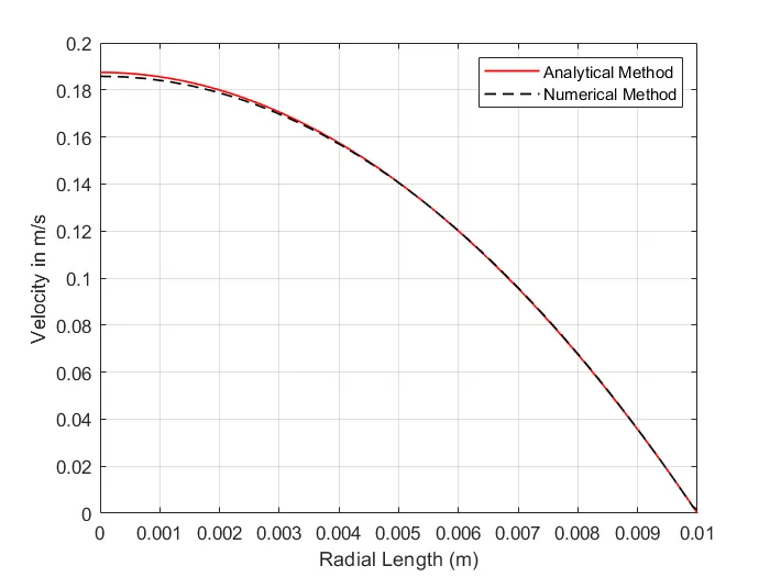
- The velocity profile of the analytical and numerical results do match accurately. With an error of less than 0.1%, the numerical results can be considered valid. The plot clearly depicts that the velocity of the flow at the walls becomes zero due to the wall shear stresses and maximum at the center of the pipe.
2. Pressure drop comparison.
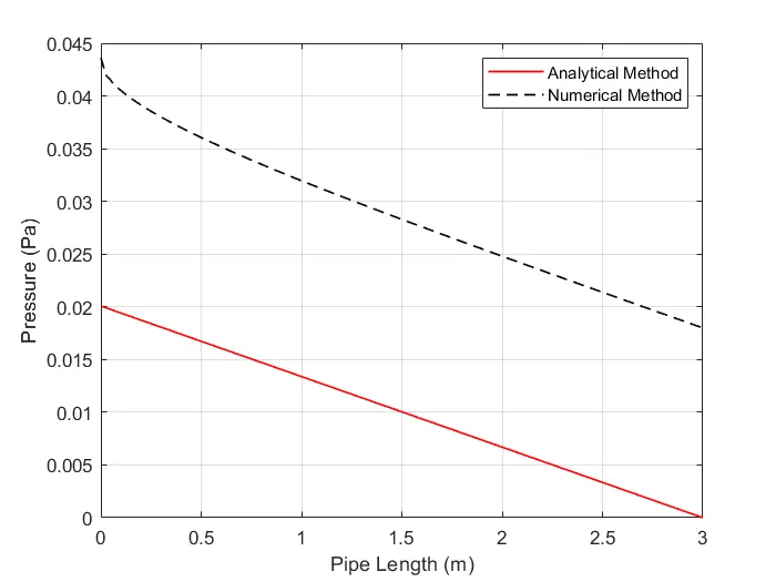
- The pressure plot for the analytical and numerical results do look parallel to each other, but it can be clearly observed that there is some difference in the pressure drop values of the analytical solution and numerical solution.
- This difference in both solutions is due to the coarse meshing in the horizontal direction. That is, along the flow direction, the meshing is very very coarse. This coarse meshing in FVM results in a high difference in the values when compared to the analytical solution.
- Although the plot shows there is a difference in the solutions, the numerical solution can be considered valid based on the meshing part as the plot illustrates that the pressure at the start of the pipe is high and becomes zero at the end of the pipe for both the solutions.
3. Shear stress comparison
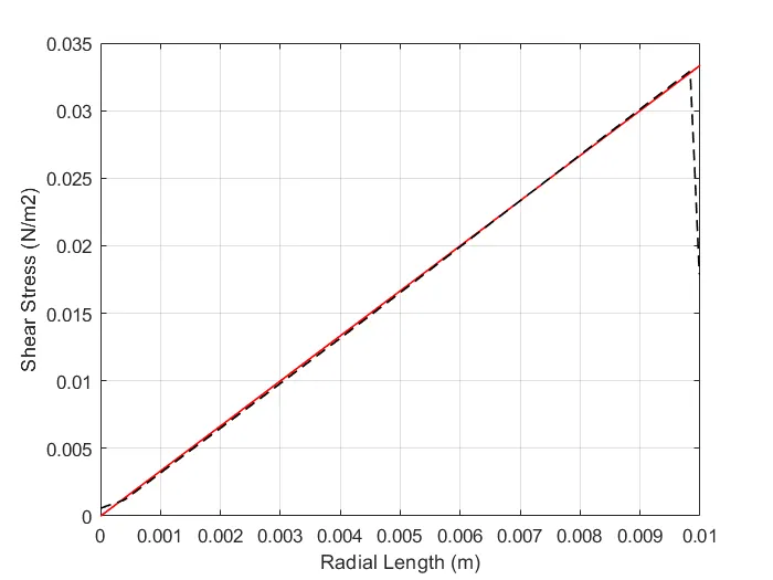
- The above plot clearly indicates the analytical and numerical solutions for wall shear stress in the flow are accurate. The numerical solution can be assumed to be precise. With an error of less than 0.1%, the numerical solution is accepted.
- The plot clearly shows that the shear stress value in the analytical solution is high at the walls of the pipe and almost equal to zero at the center of the pipe.