Week 9 - FVM Literature Review

1. Problem definition - In this problem we have to discuss the following theory -

• Finite Volume Method (FVM)
• Difference between finite volume method (FVM) and finite difference method (FDM)
• Need for interpolation scheme and flux limitors in FVM

2. Theory -

Consider a partial differential equation -

`frac{delU}{delx} = e^{x*y}`

on Integrating , we get

`U(x) = frac{e^{x*y}}{y}`

for different values of x, we can calculate U(x)

In order to find the solution at discrete space we need to convert the above partial differential equation into a form which will allow us to find the value of U at various points of x i.e into algebraic form. This process of converting the PDE into algebraic equation is called discretization

There are three methods of discretization

• Finite Volume Method (FVM)
• Finite Difference Method (FDM)
• Finite Element Method (FEM)

Finite Volume Method -

• It is a method of representing the partial differential equation into algebraic equation
• The name finite volume is because we split the entire domain into sets of control volume known as cells
• The PDE is satisfied over finite sized control volume
• Cells are of arbitary shapes
• All information is stored at geometric centroids of the cells which is called as cell centres

Difference between FVM and FDM

1. Finite Volume Method

• It is based on Integral form of governing equation
• Discretization is conducted over each control volume
• It can be directly applied to unstructured grids
• The variable values are stored at the centre of the finite volume
• It conserve quantities better and in discretize form we can read the definition mathematically

2. Finite Difference Method

• It is based on Differential form of governing equation
• Discretization is conducted at each point
• It cannot be directly applied to unstructured grids and for doing it we have to use Variable transformation approach
• The variable values are stored at nodes only
• It does not conserve quantities better than FVM and also we cannot read the definition mathematically by seeing the discretize equation

Need for Interpolation Scheme and Flux Limitors in FVM

• Interpolation Scheme

Consider 1 Dimensional steady state heat conduction equation with heat generation through a rod -

`del/(delx) (alpha*frac{delT}{delx}) + S = 0`

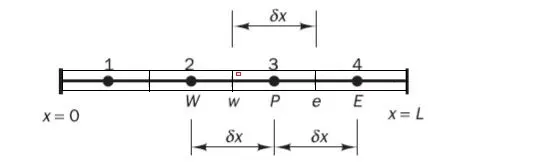
we are taking a small volume as shown in red color and we are solving the above governing equation in that small volume and integrating it over the entire domain

`int^p (del/(delx) (alpha*frac{delT}{delx}) + S) dV = 0`

This is the integral form of governing equation

`int_w^e del/(delx) (alpha*frac{delT}{delx}) dV + int_w^e S* dV = 0`

`int_w^e del/(delx) (alpha*frac{delT}{delx}) A dx + int_w^e S* dV = 0`

`[del/(delx) (alpha*frac{delT}{delx}) A]_w^e +barS*dV = 0`

`alpha_e *A*(frac{delT}{delx})_e - alpha_w *A*(frac{delT}{delx})_w + barS*dV = 0`

we can use taylor series for finding the above derivative

`alpha_e *A*(frac{T_E - T_P}{Deltax}) - alpha_w *A*(frac{T_P - T_W}{Deltax})_w + barS*dV = 0`

`alpha_e *A*(frac{T_E - T_P}{Deltax}) - alpha_w *A*(frac{T_P - T_W}{Deltax})_w + (S_u + S_p*T_p)= 0`

the first term is of east face ,second term is of west face and last term is called source term

If our source term is a function of temperature then we have to linearise it as shown in above equation

and if `alpha` is also a function of temperature we have to linearise it too

If `alpha_e` is function of temperature then we need to calculate the temperature at the right boundary of the control volume P i.e we need to calculate `T_e`

For calculating `T_e` we need some scheme which is called as interpolation scheme

Interpolation schemes are used to transform the cell centred quantities to face centres

• Flux Limitors -

`rightarrow`when we calculate gradients at the boundary of the control volume P i.e at e and w, we need to have our values bounded and it should not jump. For shock flow problem our values will jump and there is huge discontinuities and we get huge gradient value and because of this we need flux limiters

`rightarrow`We cannot have higher order accuracy without oscillation and the objective is to have highy accurate,stable and oscillation free schemes. So the flux limiters is used in such a way that the schemes gives a higher order accuracy in smooth region and first order accuracy in shock or discontinuity region