Week 7 - Simulation of a 1D Super-sonic nozzle flow simulation using Macormack Method

1. Problem definition - In this problem we have to solve Quasi 1D supersonic nozzle flow equation using Maccormack method for both conservative and non-conservative form of equation and also comparing the primitive variables(rho,T,p,v) calculated from the two forms of governing equations

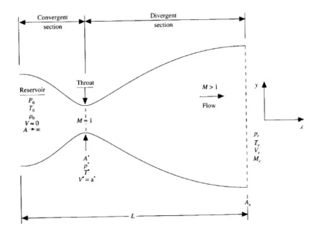figure from John D. Anderson

In this problem we will consider that inlet to the nozzle comes from a reservior and its properties is shown in figure

• Conservative form (Non - Dimensional)

Continuity equation - `frac{del(rho'*A')}{delt'} + frac{del(rho'*A'*v')}{delx'} =0`

Momentum equation - `frac{del}{delt'}(rho'*A'*v') + frac{del}{delx'}(rho'*A'*v'^2 + 1/gamma*p'*A') =1/gamma*p'*frac{delA'}{delx'}`

Energy equation - `frac{del}{delt'}(rho'*A'(frac{e'}{gamma -1} + gamma/2*v'^2)) + frac{del}{delx'}(rho'*A'*v'(frac{e'}{gamma -1} + gamma/2*v'^2)+p'*A'*v')=0`

• Non - Conservative form (Non - Dimensional)

Continuity equation - `frac{delrho'}{delt'} = -rho'*frac{delv'}{delx'} - rho'*v'*frac{dellnA'}{delx'}-v'*frac{delrho'}{delx'}`

Momentum equation - `frac{delv'}{delt'} = -v'*frac{delv'}{delx'} -1/gamma(frac{delT'}{delx'}+frac{T'}{rho'}*frac{delrho'}{delx'})`

Energy equation - `frac{delT'}{delt'} = -v'*frac{delT'}{delx'}-(gamma-1)*T'*(frac{delv'}{delx'}+v'*frac{dellnA'}{delx'})`

2. Procedure - First we will create a mesh and then provide the initial conditions for calculating the primitive variables such as density(rho),Temperature(T),pressure(p) and velocity(v) at discrete points then we will use the maccormack method to calculate the primitive variables at different time steps and finally comparing the results obtained from both conservative and non-conservative form

• Maccormack technique steps

a. Predictor step - we calculate the results using the initial condition for the first time step. In this we use forward differencing scheme for space derivative e.g `(frac{delf}{delt})_p`

where f = T,p,rho,v

b. Solution update - In this step we update the values of (f) calculated from predictor step by adding initial values to it

`f^** = f_{Initial} + (frac{delf}{delt})_p *dt`

c. Corrector step - we use the above updated values for calculating the primitive variables and in this step we use Backward differencing scheme for space derivative e.g `(frac{delf^**}{delt})_c`

d. Average time derivative - in this step we calculate the primitive variables by taking average of the values found at predictor step and corrector step

`(frac{delf}{delt})_{avg} = 0.5*(frac{delf}{delt}_p + frac{delf}{delt}_c)`

e. Calculating final updated value - In this step we add initial value with the above average time derivative value for calculating the updated values of primitive variables

`f^{end time step} = f_{Initial} + (frac{delf}{delt})_{avg} *dt`

And for conservative form , we will not use the same formula mentioned above instead we will use the generic form -

• Continuity equation

`frac{delU1}{delt'} = - frac{delF1}{delx'}`

`U1 = rho'*A'`

`F1 = rho'*A'*v'`

• Momentum equation

`frac{delU2}{delt'} = - frac{delF2}{delx'} + J2`

`U2 = rho'*A'*v'`

`F2 = rho'*A'*v'^2 + 1/gamma * p'*A'`

`J2 = 1/gamma *p'* frac{delA'}{delx'}`

• energy equation

`frac{delU3}{delt'} = - frac{delF3}{delx'}`

`U3 = rho'*A' (frac{e'}{gamma-1} + gamma/2 * v'^2)`

`F3 = rho'*A'*v' (frac{e'}{gamma-1} + gamma/2 * v'^2) + p'*A'*v'`

where U - Solution vector , F - Flux vector , J - source term

3. Theory - There are two types of governing equation namely conservative and non-conservative form and two types of control volume namely Infinitesimal and Arbitarary control volume

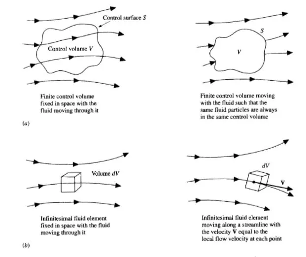figure from John D. Anderson

Conservative form - Control volume is fixed

Non - Conservative form - Control volume is moving

The above two forms are equivalent and there is no difference ,one form can be converted into another form quite easily and exactly,they both are different in world of numerical discretization

conservative form is more accurate and they tend to work well when there is discontinuities or shock existing in the domain

For solving conservative form we will not use the same exact formula mentioned above instead we will use the generic form or pure form for getting stable results

Maccormack method is an explicit finite difference technique which is second order accurate for both space and time

Also we can apply backward differencing on predictor step and forward differencing on corrector step ,the results will be the same

4. Derivations -

• Consider integral form of continuity equation

`del/(delt) intintint_Vrho*dV + intint_s rho*v*dS =0`

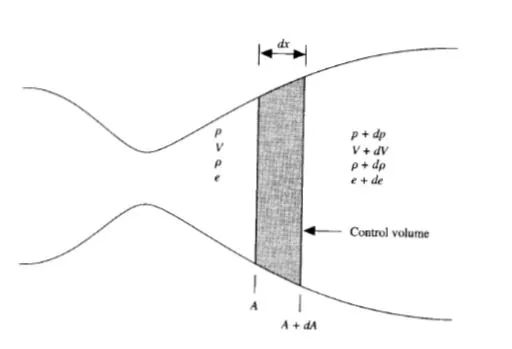figure from John D. Anderson

consider a shaded control volume , the properties at left and right of control volume is shown in above figure and the first term of the equation changes to

`del/(delt) intintint_vrho*dV = del/(delt) rho*A*dx ......(1)`

A*dx is volume of control volume of length dx

and second term of equation changes to-

`intint_s rho*v*dS = - Inflow + Outflow`

inflow is taken as negative and outflow is taken as positive

`intint_s rho*v*dS = -(rho*v*A) + (rho+drho)(v+dv)(A+dA)`

`intint_s rho*v*dS = -rho*v*A + rho*v*A +rho*v*dA + rho*dv*A +rho*dv*dA + drho*v*A + drho*v*dA + drho*dv*A + drho*dv*dA`

neglecting the terms involving the product of differentials because it is very small and cancelling the like terms

`intint_s rho*v*dS = rho*v*dA + rho*A*dv + A*v*drho`

`intint_s rho*v*dS = d(rho*A*v)`

dividing by dx

`frac{del(rho*A)}{delt} + frac{del(rho*A*v)}{delx} =0..........(2)`

This is the partial differential form of continuity equation for quasi 1D flow

Also the above form is Dimensional form and we have to use non-dimensional form

`T' = T/T_o , rho' = rho/rho_o,x' = x/L , a_o = sqrt(gamma*R*T_o) , v = v/a_o , t' = t/(L/a_o) , A' = A /A^{throat}`

where o is the properties at reservior

`rightarrow`converting the equation number (2) into conservation non-dimensional equation

`frac{del(rho*A)}{delt} + frac{del(rho*A*v)}{delx} =0`

`frac{delrho'*A'}{delt'}(rho_o*A^{throat}*a_o/L) + frac{del(rho'*A'*v')}{delx}(rho_o*A^{throat}*a_o/L) =0`

`frac{del(rho'*A')}{delt'} + frac{del(rho'*A'*v')}{delx'} =0.......(3)`

This is the non - dimensional conservative form of continuity equation for Quasi 1D supersonic nozzle flow

`rightarrow`converting the equation number (2) into non-conservation non-dimensional equation

`frac{del(rho*A)}{delt} + frac{del(rho*A*v)}{delx} =0`

on expanding the second term we get

`frac{del(rho*A)}{delt} + rho*Afrac{delv}{delx} + rho*vfrac{delA}{delx} + A*vfrac{drho}{dx} = 0`

`frac{del(rho'*A')}{delt'}(rho_o*A^{throat}*a_o/L) + rho'*A'frac{delv'}{delx'}(rho_o*A^{throat}*a_o/L) + rho'*v'frac{delA'}{delx'}(rho_o*A^{throat}*a_o/L) + A'*v'frac{drho'}{dx'}(rho_o*A^{throat}*a_o/L) = 0`

also note that area (A) is function of (x) only

`frac{del(rho'*A')}{delt'} = A' frac{delrho'}{delt'}`

Therefore our above equation reduces to -

`frac{delrho'}{delt'} = - rho'frac{delv'}{delx'} - rho'*v'frac{del(lnA')}{delx'} - v'frac{delrho'}{delx'}.......(4)`

This is the non - dimensional non-conservative form of continuity equation for Quasi 1D supersonic nozzle flow

• Consider integral form of x - component of momentum equation

`del/(delt) intintint_V (rho*u)dV + intint_s (rho*u*v) dS = - intint_s (p*dS)_x .........(5)`

consider a shaded control volume , the properties at left and right of control volume is shown in above figure and the first term of the equation changes to

`del/(delt) intintint_V(rho*u)dV = del/(delt) (rho*v*A*dx)`

Consider the second term from equation (5)

`intint_s (rho*u*v) dS = -Inflow + Outflow`

`intint_s (rho*u*v) dS = -(rho*v^2*A) + (rho+drho)(v +dv)^2(A+dA)`

inflow is taken as negative and outflow is taken as positive

consider the term on the right side of the equation

`intint_S (p*dS)_x = -p*A + (p+dp)(A+dA) - 2*p*(dA)/2`

putting all the above terms in equation (5)

`frac{del(rho*v*A*dx)}{delt} -(rho*v^2*A) + (rho+drho)(v +dv)^2(A+dA) = p*A - (p+dp)(A+dA) + p*dA`

cancelling same terms and ignoring products of differentials,we get

`frac{del(rho*v*A*dx)}{delt} + del(rho*v^2*A) = -A*delp`

dividing the above equation by dx

`frac{del(rho*v*A)}{delt} + frac{del(rho*v^2*A)}{delx} = -Afrac{delp}{delx} ...........(6)`

The above equation is in conservation form ,converting the above form into non - conservation form

Multiplying the continuity eqation i.e eq (1) by velocity (v)

`v*frac{del(rho*A)}{delt} +v* frac{del(rho*A*v)}{delx} =0`

substracting the above equation with equation (3) , we get

`frac{del(rho*v*A)}{delt} - v*frac{del(rho*A)}{delt} + frac{del(rho*v^2*A)}{delx} -v* frac{del(rho*v*A)}{delx} = -A*frac{delp}{delx}`

on cancelling the same terms and expanding, we get

`rho*Afrac{delv}{delt} + rho*A*vfrac{delv}{delx} = - Afrac{delp}{delx}`

`rhofrac{delv}{delt} + rho*vfrac{delv}{delx} = - frac{delp}{delx}........(7)`

also we know that `p = rho*R*T`

where p - pressure , T - temperature and R is characteristics gas constant

on derivating with respect to x , we get

`frac{delp}{delx} = R(rho*frac{delT}{delx} + T*frac{delrho}{delx})`

putting the above formula in equation (7) , we get

`rhofrac{delv}{delt} + rho*vfrac{delv}{delx} = - R(rho*frac{delT}{delx} + T*frac{delrho}{delx}).......(8)`

The above equation is the momentum equation in non - conservation dimensional form for 1D supersonic nozzle flow

`rightarrow`converting the equation(8) in non - dimensional non - conservation form

`rho'frac{delv'}{delt'}(rho_o*a_o^2/L) + rho'*v'frac{delv'}{delx'}(rho_o*a_o^2/L) = - R(rho'*frac{delT'}{delx'} + T'*frac{delrho'}{delx'})(rho_o*T_o/L)`

OR

`rho'frac{delv'}{delt'}= - rho'*v'frac{delv'}{delx'} - (rho'*frac{delT'}{delx'} + T'*frac{delrho'}{delx'})(R*T_o/a_o^2)`

`frac{R*T_o}{a_o^2} = frac{gamma*R*T_o}{gamma*a_o^2} = frac{a_o^2}{gamma*a_o^2} = 1/gamma`

`frac{delv'}{delt'}= -v'frac{delv'}{delx'} - 1/gamma(frac{delT'}{delx'} + frac{T'}{rho'}*frac{delrho'}{delx'}).......(9)`

The above equation is the momentum equation in non - conservation non - dimensional form for 1D supersonic nozzle flow

`rightarrow` converting equation (6) into conservation non - dimensional form of Quasi 1D supersonic nozzle flow

`frac{del(rho*v*A)}{delt} + frac{del(rho*v^2*A)}{delx} = -Afrac{delp}{delx}`

Also we can convert the right side of above equation to -

`frac{del(p*A)}{delx} = p*frac{del(A)}{delx} + A*frac{del(p)}{delx}`

`- A*frac{del(p)}{delx} = p*frac{del(A)}{delx} - frac{del(p*A)}{delx}`

putting this above equation -

`frac{del(rho'*v'*A')}{delt'}(rho_o*a_o^2*A^(throat)/L) + frac{del(rho'*v'^2*A')}{delx'}(rho_o*a_o^2*A^(throat)/L) = p'*frac{del(A')}{delx'}(rho_o*R*T_o*A^(throat)/L) - frac{del(p'*A')}{delx'}(rho_o*R*T_o*A^(throat)/L)`

on simplifying above eqaution we get and putting `frac{R*T_o}{a_o^2} = 1/gamma`

`frac{del(rho'*v'*A')}{delt'} + frac{del(rho'*v'^2*A' + 1/gamma*p'*A')}{delx'} = 1/gamma * p' * frac{delA'}{delx'}..........(10)`

This is the equation for conservative non - dimensional form for supersonic 1D nozzle flow

• consider integral form of energy equation

`del/(delt) intintint_V (rho*(e + v^2/2))*dV + intint_S (rho*(e + v^2/2))*v*dS = - intint_S (p*v)*dS.........(11)`

Doing the same step as mentioned above we get the following equation

`rho*frac{dele}{delt} + rho*v*frac{dele}{delx} = -p*frac{delv}{delx} - p*v*frac{del(lnA)}{delx}`

putting `e = C_v*T ,p = rho*R*T` in above equation,we get

`rho*C_v*frac{delT}{delt} + rho*v*C_v*frac{delT}{delx} = - rho*R*T(frac{delv}{delx} + v*frac{del(lnA)}{delx})`

also `R/gamma = frac{R}{R/(gamma-1)} = gamma -1` and converting it into non - dimensional form

The equation reduces to -

`frac{delT'}{delt'} = - v'*frac{delT'}{delx'} - (gamma - 1)*T'*(frac{delv'}{delx'} + v'*frac{del(lnA')}{delx'}).........(12)`

The above equation is the energy equation in non - conservation non - dimensional form for 1D supersonic nozzle flow

5. Code -

Main code -

clear all
close all
clc

%creating mesh
nx = 31;
x = linspace(0,3,nx);
dx = x(2) - x(1);
gamma = 1.4 ; 
C = 0.5;

%number of time steps
nt = 1400;



%function calling for conservative and non-conservative form 

[Density_1 Temperature_1 Pressure_1 Mach_number_1 U2_array_1 ] = nozzle_non_conservative(nx,x,dx,gamma,C,nt)

[Density_2 Temperature_2 Pressure_2 Mach_number_2 U2_array_2] = nozzle_conservative(nx,x,dx,gamma,C,nt)

%plotting of results
figure(5);
plot(x,Density_1,'LineWidth',2);
hold on
plot(x,Density_2,'*','LineWidth',2);
xlabel('Domain length (x)');
ylabel('Density (rho)');
legend('Non-Conservative','Conservative');

figure(6);
plot(x,Temperature_1,'LineWidth',2);
hold on
plot(x,Temperature_2,'*','LineWidth',2);
xlabel('Domain length (x)');
ylabel('Temperature (T)');
legend('Non-Conservative','Conservative');

figure(7);
plot(x,Pressure_1,'LineWidth',2);
hold on
plot(x,Pressure_2,'*','LineWidth',2);
xlabel('Domain length (x)');
ylabel('Pressure (p)');
legend('Non-Conservative','Conservative');

figure(8);
plot(x,Mach_number_1,'LineWidth',2);
hold on
plot(x,Mach_number_2,'*','LineWidth',2);
xlabel('Domain length (x)');
ylabel('Mach_number (M)');
legend({'Non-Conservative','Conservative'},'Location','Northwest');

figure(9);
plot(x,U2_array_1,'color','b','LineWidth',2);
hold on 
plot(x,U2_array_2,'color','g','LineWidth',2);
title_text = sprintf('Mass flow rate across the domain for conservative and non-conservative form');
title(title_text)
xlabel('Length of domain');
ylabel('mass flow rate');
legend({'Non-Conservative','Conservative'},'Location','Northwest');

calling of function by non - conservative form

function  [rho T p M U2] = nozzle_non_conservative(nx,x,dx,gamma,C,nt)


%initial conditions
rho = 1 - 0.3146*x;
T = 1 - 0.2314*x;
v = (0.1 + 1.09*x).*T.^0.5;
A = 1 + 2.2*(x - 1.5).^2;
m_initial = rho.*v.*T ;


for k = 1 : nt
  
    rho_old = rho ;
    v_old = v ;
    T_old = T ;   
    
   %Calculating adaptive time step
    dt_array(k) = min(C*dx./(sqrt(T)+v));
    dt = dt_array(k);

        %predictor step
        
        for i = 2 : nx-1
           
           drhodx = (rho(i+1)-rho(i))/dx ;
           dvdx = (v(i+1)-v(i))/dx ;
           dTdx = (T(i+1)-T(i))/dx ;
           dlogAdx = (log(A(i+1))-log(A(i)))/dx ;
           
           %continuity equation
           drhodt_p(i) = - rho(i)*dvdx - rho(i)*v(i)*dlogAdx - v(i)*drhodx ;
           
           %momentum equation
           dvdt_p(i) = - v(i)*dvdx - (1/gamma) * (dTdx + ((T(i)/rho(i)) * drhodx)) ;
           
           %energy equation
           dTdt_p(i) = - v(i)*dTdx - (gamma - 1)*T(i)*(dvdx + (v(i)*dlogAdx)) ; 
  
  
           %solution update
           rho(i) = rho(i) + drhodt_p(i) * dt ;
           v(i) = v(i) + dvdt_p(i) *dt ;
           T(i) = T(i) + dTdt_p(i) *dt ;
  
        end
     
     
     
        %corrector step
        

        for j = 2 : nx-1
          
          drhodx = (rho(j)-rho(j-1))/dx ;
          dvdx = (v(j)-v(j-1))/dx ;
          dTdx = (T(j)-T(j-1))/dx ;
          dlogAdx = (log(A(j))-log(A(j-1)))/dx ;
   
           %continuity equation
           drhodt_c(j) = - rho(j)*dvdx - rho(j)*v(j)*dlogAdx - v(j)*drhodx ;
           
           %momentum equation
           dvdt_c(j) = - v(j)*dvdx - 1/gamma * (dTdx + (T(j)/rho(j) * drhodx)) ;
           
           %energy equation
           dTdt_c(j) = - v(j)*dTdx - (gamma - 1)*T(j)*(dvdx + (v(j)*dlogAdx)) ; 
           
        end
     
     %computing average time derivative
      drhodt = 0.5*(drhodt_p + drhodt_c);
      dvdt = 0.5*(dvdt_p + dvdt_c);
      dTdt = 0.5*(dTdt_p + dTdt_c);
     
     %final solution update
     for l = 2 : nx-1
       
        rho(l) = rho_old(l) + drhodt(l)*dt;
        v(l) = v_old(l) + dvdt(l)*dt;
        T(l) = T_old(l) + dTdt(l)*dt;
        
     end
     
     
     
     %inlet condition
     v(1) = 2*v(2) - v(3) ;
     
     %outlet condition
     rho(nx) = 2*rho(nx-1) - rho(nx-2);
     v(nx) = 2*v(nx-1) - v(nx-2);
     T(nx) = 2*T(nx-1) - T(nx-2);
     
     %calculating pressure and mach number using above values
     for i = 1: nx
       
       p(i) = rho(i)*T(i);
       M(i) = v(i)/sqrt(T(i));
       U2(i) = rho(i)*A(i)*v(i);
       
     end  
     
    
     
 
     
     if  k==50 || k ==100 || k==200 || k==400 || k==800
       
         
       figure(3)
       plot(x,m_initial,x,U2,'LineWidth',2);
       hold on
       xlabel('Domain length (x)');
       ylabel('Mass flow rate');
       title_text = sprintf('Mass flow rate at different time step across the domain for non-conservative form');
       title(title_text)
       
       if k == 800
             legend('nt=0','nt = 50','nt = 100','nt = 200','nt = 400','nt = 800');
       end 
          
         
       
     end  
     
      

figure(1);
subplot(2,2,1);
plot(k,rho((nx+1)/2),'color','b','*','LineWidth',2);
hold on
title_text = sprintf('time step = %d',k);
title(title_text)
pause(0.001)
xlabel('Number of time steps (nt)');
ylabel('Density at throat (rho)');
legend('Non-Conservative');

figure(1);
subplot(2,2,2);
plot(k,T((nx+1)/2),'color','g','*','LineWidth',2);
hold on
title_text = sprintf('time step = %d',k);
title(title_text)
pause(0.001)
xlabel('Number of time steps (nt)');
ylabel('Temperature at throat (T)');
legend('Non-Conservative');

figure(1);
subplot(2,2,3);
plot(k,p((nx+1)/2),'color','m','*','LineWidth',2);
hold on
title_text = sprintf('time step = %d',k);
title(title_text)
pause(0.001)
xlabel('Number of time steps (nt)');
ylabel('Pressure at throat (p)');
legend('Non-Conservative');

figure(1);
subplot(2,2,4);
plot(k,M((nx+1)/2),'color','k','*','LineWidth',2);
hold on
title_text = sprintf('time step = %d',k);
title(title_text)
pause(0.001)
xlabel('Number of time steps (nt)');
ylabel('Mach number at throat (M)');
legend('Non-Conservative');



end
     

     


endfunction

calling of function by conservative form

function  [rho T p M U2] = nozzle_conservative(nx,x,dx,gamma,C,nt)


%initial condition
A = 1 + 2.2*(x - 1.5).^2;



for i = 1:nx
  
  if (x(i)<= 0.5)
    
    rho(i) = 1;
    T(i) = 1;
    
  elseif (x(i)> 0.5 && x(i)<= 1.5)   
    
    rho(i) = 1 - 0.366*(x(i) - 0.5);
     T(i) = 1 - 0.167*(x(i) - 0.5);
     
   else
     
    rho(i) = 0.634 - 0.3879*(x(i) - 1.5);
     T(i) = 0.833 - 0.3507*(x(i) - 1.5);
     
  end  
  
  v(i) = 0.59/(rho(i)*A(i)) ;
  
end  

for i = 1 :nx
  
%initial condition for solution vector
U1(i) = rho(i) * A(i) ;
U2(i) = rho(i) * A(i) * v(i) ;
U3(i) = rho(i)* A(i) * ((T(i)/(gamma-1)) + (0.5*gamma*v(i)^2)) ;

end

m_initial = U2 ;
%time loop

for k = 1 : nt
  
  % Calculating adaptive time step
  dt_array(k) = min(C*dx./(sqrt(T)+v));
  dt = dt_array(k);

      %storing old values for comparison
       U1_old = U1 ;
       U2_old = U2 ;
       U3_old = U3 ;
       
      %initial condition for flux vectorize
      for i = 1:nx
        
        F1(i) =  U2(i) ;
        F2(i) = (U2(i)^2/U1(i)) + ((gamma-1)/gamma) * (U3(i)- 0.5*gamma*U2(i)^2/U1(i)) ;
        F3(i) = (gamma*U2(i)*U3(i))/U1(i) - (0.5*gamma*(gamma-1)*U2(i)^3/U1(i)^2) ;
        
      end
              
     
     %predictor step
               
       for i = 2:nx-1
         
         J2(i) = 1/gamma * rho(i)*T(i)*(A(i+1)-A(i))/dx;
           
             
           dU1dt_p(i) = - (F1(i+1) - F1(i))/dx ;
           
           dU2dt_p(i) = - (F2(i+1) - F2(i))/dx + J2(i) ;
           
           dU3dt_p(i) = - (F3(i+1) - F3(i))/dx ;
           
           
           %solution update
           U1(i) = U1(i) + dU1dt_p(i)*dt ;
           U2(i) = U2(i) + dU2dt_p(i)*dt ;
           U3(i) = U3(i) + dU3dt_p(i)*dt ;
           

        end
      
     %calculating primitive variables from above solution vector
     for i = 1:nx
       rho(i) = U1(i)/A(i) ;
       v(i) = U2(i)/U1(i) ;
       T(i) = (gamma-1)*(U3(i)/U1(i) - (0.5*gamma*v(i)^2)) ;
     end

     
       %initial condition for flux vector for corrector step
       for i = 1:nx
       
        F1(i) =  U2(i) ;
        F2(i) = (U2(i)^2/U1(i)) + ((gamma-1)/gamma) * (U3(i)-0.5*gamma*U2(i)^2/U1(i)) ;
        F3(i) = (gamma*U2(i)*U3(i))/U1(i) - (0.5*gamma*(gamma-1)*U2(i)^3/U1(i)^2) ;
        
      end        
       
       
       %corrector step 
       
       for j = 2:nx-1
         
         J2(j) = 1/gamma * rho(j)*T(j)*(A(j)-A(j-1))/dx;  
         
            
           dU1dt_c(j) = - (F1(j) - F1(j-1))/dx ;
           
           dU2dt_c(j) = - (F2(j) - F2(j-1))/dx + J2(j) ;
           
           dU3dt_c(j) = - (F3(j) - F3(j-1))/dx ;
           
       end
       
       %computing average time derivative
       dU1dt = 0.5*(dU1dt_p + dU1dt_c) ;
       dU2dt = 0.5*(dU2dt_p + dU2dt_c) ;
       dU3dt = 0.5*(dU3dt_p + dU3dt_c) ;
               
       %final solution update
       for l = 2:nx - 1
         
           U1(l) = U1_old(l) + dU1dt(l)*dt ;
           U2(l) = U2_old(l) + dU2dt(l)*dt ;
           U3(l) = U3_old(l) + dU3dt(l)*dt ;
          
       end  
       
       %inlet condition
       U1(1) = rho(1)*A(1) ;
       U2(1) = 2*U2(2) - U2(3) ;
       v(1) = U2(1)/U1(1) ;
       U3(1) = U1(1)*((T(1)/(gamma - 1)) + (0.5*gamma*v(1)^2));
               
               
       %outflow condition
       U1(nx) = 2*U1(nx-1) - U1(nx-2) ;
       U2(nx) = 2*U2(nx-1) - U2(nx-2) ;
       U3(nx) = 2*U3(nx-1) - U3(nx-2) ;
       
       %calculating the final primitive variables 
       for i = 1:nx
         
           rho(i) = U1(i)/A(i) ;
            v(i) = U2(i)/U1(i) ;
            T(i) = (gamma-1)*(U3(i)/U1(i) - (0.5*gamma*v(i)^2)) ;
            p(i) = rho(i)*T(i);
            M(i) = v(i)/sqrt(T(i));
            
       end
     
     
     
     if  k==50 || k ==100 || k==200 || k==400 || k==800
       
         
       figure(4);
       plot(x,m_initial,x,U2,'LineWidth',2);
       hold on
       xlabel('Domain length (x)');
       ylabel('Mass flow rate');
       title_text = sprintf('Mass flow rate at different time step across the domain for conservative form');
       title(title_text)
       
       if k == 800
             legend('nt=0','nt = 50','nt = 100','nt = 200','nt = 400','nt = 800');
       end 
          
         
       
     end  

figure(2);
subplot(2,2,1);
plot(k,rho((nx+1)/2),'color','b','*','LineWidth',1);
hold on
title_text = sprintf('time step = %d',k);
title(title_text)
pause(0.001)
xlabel('Number of time steps (nt)');
ylabel('Density at throat (rho)');
legend('Conservative');

figure(2);
subplot(2,2,2);
plot(k,T((nx+1)/2),'color','g','*','LineWidth',1);
hold on
title_text = sprintf('time step = %d',k);
title(title_text)
pause(0.001)
xlabel('Number of time steps (nt)');
ylabel('Temperature at throat (T)');
legend('Conservative');

figure(2);
subplot(2,2,3);
plot(k,p((nx+1)/2),'color','m','*','LineWidth',1);
hold on
title_text = sprintf('time step = %d',k);
title(title_text)
pause(0.001)
xlabel('Number of time steps (nt)');
ylabel('Pressure at throat (p)');
legend('Conservative');

figure(2);
subplot(2,2,4);
plot(k,M((nx+1)/2),'color','k','*','LineWidth',1);
hold on
title_text = sprintf('time step = %d',k);
title(title_text)
pause(0.001)
xlabel('Number of time steps (nt)');
ylabel('Mach number at throat (M)');
legend('Conservative');


     
end


endfunction 

6. Results -

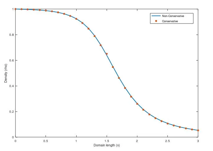
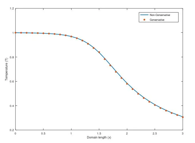
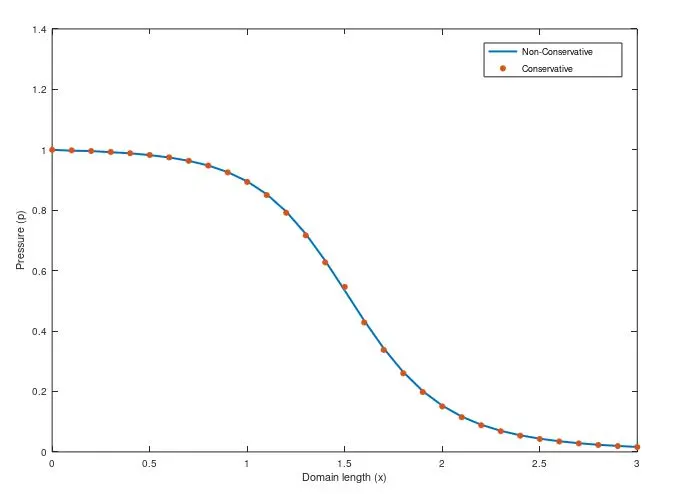
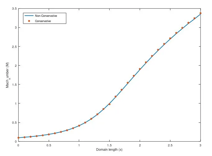
• variation of density(rho), pressure(p), temperature(T), and mach number(M) with respect to domain length (x)

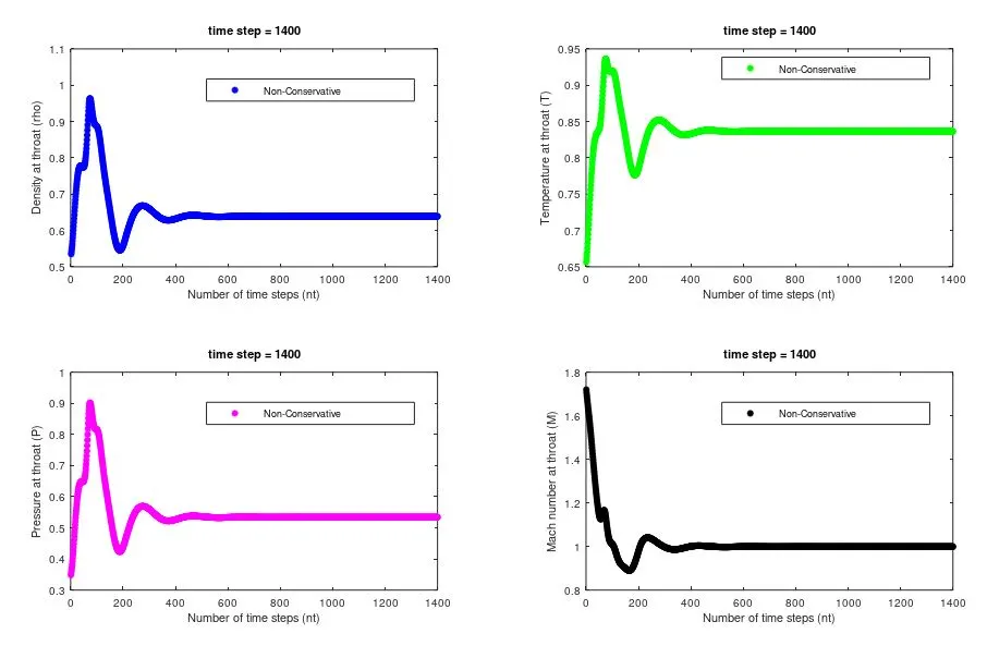
• variation of density(rho), pressure(p), temperature(T), and mach number(M) with number of time steps (nt) at the throat of the nozzle for non - conservative form

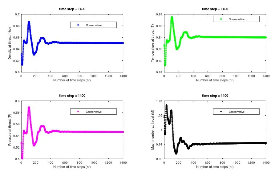
• variation of density(rho), pressure(p), temperature(T), and mach number(M) with number of time steps (nt) at the throat of the nozzle for conservative form

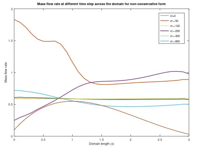
• variation of mass flow rate at different time steps (nt) across the domain length(x) for non - conservative form

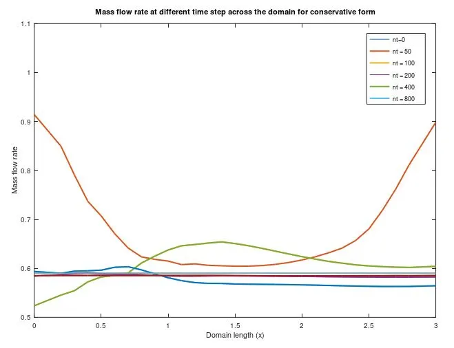
• variation of mass flow rate at different time steps (nt) across the domain length(x) for conservative form

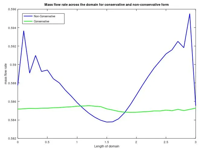
• variation of mass flow rate across the domain length (x) for conservative and non - conservative form

7 - Conclusion -

• The results are same for both conseravtive and non - conservative form
• The variation of primitive variables such as density ,temperature ,pressure and velocity across the domain length(x) is same for both conservative and non-conservative form
• The variation of primitive variables such as density ,temperature ,pressure and velocity for different time steps(nt) is same for both conservative and non-conservative form
• As we increase the number of time steps , the mass flow rate is becoming constant for both conservative and non - conservative form
• The mass flow rate at the throat is less fluctuating in conservtive form then the non - conservative form
• The reason for using the non - dimensional form for solving the above problem is that the primitive variables will vary between 0 and 1 and there will be ease in presenting the results
• The reason for using different initial condition for conservative and non - conservative form is that our solution should converge faster as we will are using the generic/pure form for solving the conservative form
• For our solution to be stable coutant number should be less than or equal to 1 `frac{dt*(a + v)}{dx}`
• If flux vector(F) is specified in terms of primitive variables (rho,T,p,M) then instabilities will occur during the time - marching solution and hence we have specified flux vector in terms of solution vector(U)