Week 5 - Mid term project - Solving the steady and unsteady 2D heat conduction problem

1. Problem definition - In this problem we have to solve the steady and unsteady state heat conduction equation using both implicit and explicit approach.The general 2 Dimensional heat conduction equation is

`frac{deltaT}{deltat} = alpha (frac{delta^2T}{deltax^2} + frac{delta^2T}{deltay^2} )`

We will solve for two cases -

• Transient / Unsteady state equation

`frac{deltaT}{deltat} = alpha (frac{delta^2T}{deltax^2} + frac{delta^2T}{deltay^2} )`

• Steady state equation

`(frac{delta^2T}{deltax^2} + frac{delta^2T}{deltay^2} ) = 0`

In this problem we will assume a plane wall of 10x10 matrix and specify the temperature values at all the sides of the wall as boundary conditions and calculate the temperature distribution at inner nodes. After solving we will plot the temperature distribution for each and every case and approach.

2. Procedure - First we will solve for steady state using implicit approach as in this case we will have system of linear equation and we will use iterative solver like Jacobi,Gauss Seidel and Successive over relaxation method for computing the temperature values. After this we will solve for unsteady state heat equation using both implicit and explicit approach.For Explicit equation we dont need any solver because the value on the RHS of the equation is known all we have to do is just insert the value and get the answer but in case of Implicit equation we have to use a time marching solution concept in addition to it, an iterative solver is also used to solve the system of linear equations.

3. Theory - We can solve the system of linear equation using direct method which can solve the equation in fixed number of steps but it is quite inefficient, so we use fixed point method

Iterative solver is used to solve the system of linear equations and there are three types of solver Jacobi, Gauss Seidel and SOR method.In all this method we initially make a guess value and we assume that it is the solution to my linear equation and based on the residue (error) value we compute a new array of guess value and we iterate like this until we reached the converge results

The basic difference between jacobi and gauss seidel method is that in jacobi it uses the same old guess values throughout the iteration whereas in gauss seidel method it uses the updated guess values for each iterations

The Successive over relaxation method (SOR) is a wrapper which is applied on jacobi or gauss seidel for improved performance

In this we will use a function calling command for both steady and unsteady state while writing a code

Also for transient condition we will use time marching solution concept

Time marching solution is used when our PDEs contain time derivative ,so in this problem we will use in transient state

4. Equations - The equation for steady and unsteady state using implicit and explicit approach are given below

• For steady state implicit equation - `T(i,j) = 1/k (frac{Told(i+1,j)+Told(i-1,j)}{dx^2} + frac{Told(i,j+1)+Told(i,j-1)}{dy^2} )`

where `k = frac{2(dx^2 + dy^2)}{dx^2*dy^2}`

• For unsteady state explicit equation - `T_(i,j)^(n+1) = T_(i,j)^n + alpha*deltat(frac{T_(i+1,j)^n - 2*T_(i,j)^n + T_(i-1,j)^n}{dx^2} + frac{T_(i,j+1)^n - 2*T_(i,j)^n + T_(i,j-1)^n}{dy^2})`

• For unstaedy state implicit equation - `T_(i,j)^(n+1) = frac{T_(i,j)^n + k1(T_(i+1,j)^(n+1) + T_(i-1,j)^(n+1)) + k2(T_(i,j+1)^(n+1) + T_(i,j-1)^(n+1))}{(1 + 2k1 +2k2)}`

where `k1 = frac{alpha*dt}{dx^2}`

`k2 = frac{alpha*dt}{dy^2}`

• For SOR method - `T_(i,j) = (1-alpha)*Told(i,j) + alpha*(T_(jacobi) or T_(gs))`

5. Code -

• For steady state

clear all
close all 
clc 

%solving a 2D steady state heat conduction equation
%d^2(T)/dx^2 + d^2(T)/dy^2 = 0

%number of grid points
nx = ny = 10;

%assigning BCs
T = 300*ones(10,10);
T(1,:) = 600;
T(end,:) = 900;
T(:,1) = 400;
T(:,end) = 800;
T(1,1) = 500;
T(1,end) = 700;
T(end,1) = 650;
T(end,end) = 850;
Told = T;



%initializing a variable
error = 9e9;
tol = 1e-4;

%function calling
steady_state_jacobi(error,tol,nx,ny,Told);
steady_state_gs(error,tol,nx,ny,Told);
steady_state_SOR(error,tol,nx,ny,Told);

calling of function - using jacobi iterative solver

function [ T ] = steady_state_jacobi(error,tol,nx,ny,Told)
  
%creating mesh
x = linspace(0,1,nx);
y = x;
dx = x(2) - x(1);
dy = dx;
T_jacobi = Told ;

%Jacobi method

  jacobi_iter = 1;
  
  k = 2*(dx^2+dy^2)/(dx^2 * dy^2);
 
  %convergence loop
  while(error > tol)
    
    %space loop
      for i = 2:nx-1
       
          for j = 2:ny-1
            
                term1 = (Told(i+1,j) + Told(i-1,j))/(dx^2);
                term2 = (Told(i,j+1) + Told(i,j-1))/(dy^2);
                        
                T_jacobi(i,j) = term1/k + term2/k ; 
                  
          end
        
      end
    
    %calculating error
    error = max(max(abs(Told - T_jacobi)));
    %updating the value
    Told = T_jacobi;
    jacobi_iter = jacobi_iter + 1;
   
    %plotting of results
    figure(1);
    contourf(T_jacobi,20);
    set(gca,'yDIR','reverse');
    colorbar;
    title_text = sprintf('Jacobi iteratons = %d',jacobi_iter);
    title(title_text)
    xlabel('x');
    ylabel('y');
    pause(0.3)
    
  end 
  
endfunction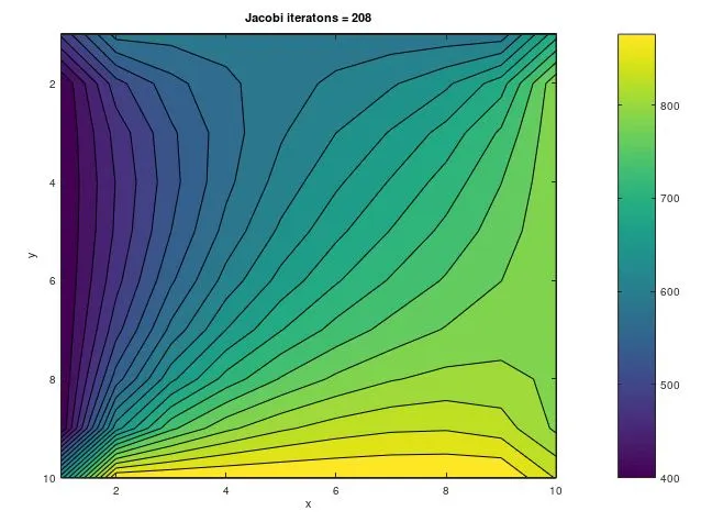

calling of function - using gauss seidel iterative solver

function [ T ] = steady_state_gs(error,tol,nx,ny,Told)
  
%creating mesh
x = linspace(0,1,nx);
y = x;
dx = x(2) - x(1);
dy = dx;
T_gs = Told ;

%gauss seidel method
  
  k = 2*(dx^2+dy^2)/(dx^2 * dy^2);

  gs_iter = 1;
  
  %convergence loop
  while(error > tol)
    
      %space loop
      for i = 2:nx-1
       
          for j = 2:ny-1
             
                 term3 = (Told(i+1,j) + T_gs(i-1,j))/(dx^2);
                 term4 = (Told(i,j+1) + T_gs(i,j-1))/(dy^2);
                 
                 
                 T_gs(i,j) = term3/k + term4/k ; 
                  
          end
        
      end
    
    %calculating error 
    error = max(max(abs(Told - T_gs)));
    %updating the value
    Told = T_gs;
    gs_iter = gs_iter + 1;
   
    %plotting of results
    figure(2);
    contourf(T_gs,10);
    set(gca,'yDIR','reverse');
    colorbar;
    title_text = sprintf('GS iteratons = %d',gs_iter);
    title(title_text)
    xlabel('x');
    ylabel('y');
    pause(0.03)
    
  end 
  
endfunction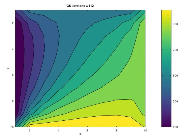

calling of function - using successive over relaxation iterative solver

function [ T ] = steady_state_SOR(error,tol,nx,ny,Told)
  
%creating mesh
x = linspace(0,1,nx);
y = x;
dx = x(2) - x(1);
dy = dx;
T_SOR = Told ;
T_gs = Told ;

alpha = 1.2;

%successive over relaxation method

  k = 2*(dx^2+dy^2)/(dx^2 * dy^2);
  
  sor_iter = 1;
  
  %convergence loop
  while(error > tol)
    
      %space loop
      for i = 2:nx-1
       
          for j = 2:ny-1
             
                 term5 = (Told(i+1,j) + T_gs(i-1,j))/(dx^2);
                 term6 = (Told(i,j+1) + T_gs(i,j-1))/(dy^2);
                 
                 
                 T_gs(i,j) = term5/k + term6/k ;
                 
                 T_SOR(i,j) = Told(i,j)*(1-alpha) + alpha*(T_gs(i,j));
                  
          end
        
      end
    
    %calculating error values
    error = max(max(abs(Told - T_SOR)));
    %updating values
    Told = T_SOR;
    sor_iter = sor_iter + 1;
    
    %plotting the results
    figure(3);
    contourf(T_SOR,20);
    set(gca,'yDIR','reverse');
    colorbar;
    title_text = sprintf('SOR iteratons = %d',sor_iter);
    title(title_text)
    xlabel('x');
    ylabel('y');
    pause(0.3)
    
  end 
   


endfunction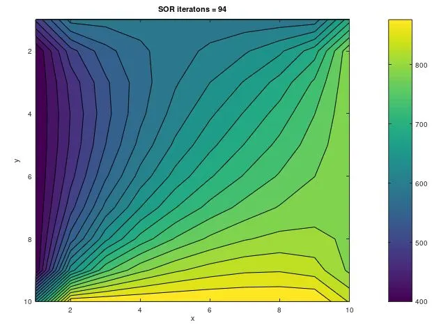

• For unsteady state - Explicit approach

clear all
close all 
clc 

%solving a 2D steady state heat conduction equation
%d^2(T)/dx^2 + d^2(T)/dy^2 = 0

%number of grid points
nx = ny = 10;

%creating mesh
x = linspace(0,1,nx);
y = x ;
dx = x(2) - x(1) ;
dy = dx ;
alpha = 1.4 ;
dt = 1e-4 ;

%assigning BCs
T = 300*ones(10,10);
T(1,:) = 600;
T(end,:) = 900;
T(:,1) = 400;
T(:,end) = 800;
T(1,1) = 500;
T(1,end) = 700;
T(end,1) = 650;
T(end,end) = 850;
Told = T;

%number of time steps
nt = 1400;

%calculating constants
k1 = (alpha*dt)/dx^2 ;
k2 = (alpha*dt)/dy^2 ;

%time loop
  
  for k = 1:nt
  
    %space loop
     for i = 2:nx-1
       
          for j = 2:ny-1
    
               T(i,j) = Told(i,j) + k1*(Told(i+1,j) - 2*Told(i,j) + Told(i-1,j)) + k2*(Told(i,j+1) - 2*Told(i,j) + Told(i,j-1));

          end
     end
  
    %updating the velocity
    Told = T;
    
    %plotting the results
    figure(1);
    contourf(T,20);
    colorbar;
    set(gca,'yDIR','reverse');
    title_text = sprintf('Transient heat conduction using explicit equation');
    title(title_text)
    xlabel('x');
    ylabel('y');
    pause(0.3)
    
  
  end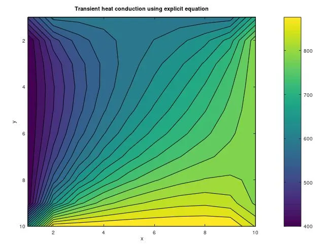

• For unsteady state - Implicit approach

clear all
close all 
clc 

%solving a 2D unsteady state heat conduction equation
%alpha*(d^2(T)/dx^2 + d^2(T)/dy^2) = dT/dt

%number of grid points
nx = ny = 10;

%creating mesh
x = linspace(0,1,nx) ;
y = x ;
dx = x(2) - x(1) ;
dy = dx ;

%specifying constant values
alpha = 1.4 ;
dt = 1e-4 ;

%assigning BCs
T = 300*ones(10,10);
T(1,:) = 600;
T(end,:) = 900;
T(:,1) = 400;
T(:,end) = 800;
T(1,1) = 500;
T(1,end) = 700;
T(end,1) = 650;
T(end,end) = 850;
Told = T;
T_previous_nt = Told ;


%initializing a variable
error = 1000;
tol = 1e-4;

%calculating constants
k1 = (alpha*dt)/dx^2 ;
k2 = (alpha*dt)/dy^2 ;
term1 = 1/(1 + 2*k1 +2*k2);
term2 = k1 * term1 ;
term3 = k2 * term1 ;

%number of time steps
nt = 1000;

transient_implicit_jacobi(nt,error,tol,nx,ny,T,Told,T_previous_nt,term1,term2,term3);
%transient_implicit_gs(nt,error,tol,nx,ny,T,Told,T_previous_nt,term1,term2,term3);
%transient_implicit_SOR(nt,error,tol,nx,ny,T,Told,alpha,T_previous_nt,term1,term2,term3)

calling of function - using jacobi iterative solver

function [ T ] = transient_implicit_jacobi(nt,error,tol,nx,ny,T,Told,T_previous_nt,term1,term2,term3)
  
Told = T;
T_previous_nt = Told ;
  
  
  
%time loop
  
  for k = 1:nt
  
     while(error > tol)
   
         %space loop
         for i = 2:nx-1
       
                for j = 2:ny-1
                     
                     H = Told(i+1,j) + Told(i-1,j);
                     V = Told(i,j+1) + Told(i,j-1);
                     
                     T(i,j) = (term1*T_previous_nt(i,j)) + (term2*H) + (term3*V) ;

                end
              
         end
  
    %updating the velocity and calculating the error
    error = max(max(abs(T - Told))) ;
    Told = T;
    
    
     end  
   
   %updating error value
   error = 1000;
   %calculating the residue
   error1 = max(max(abs(T - T_previous_nt)));
   %updating the tempertaure value for next time steps
   T_previous_nt = T ;
   
   %plotting the result for error with respect to nt
   figure(1);
   semilogy(k,error1,'marker','*','color','b');
   hold on;
   xlabel('number of time steps (nt)');
   ylabel('error(residue)');
   pause(0.001)
   
    
  end

    %plotting the results for tempertaure distribution
    figure(2);
    contourf(T,20);
    colorbar;
    set(gca,'yDIR','reverse');
    title_text = sprintf('Transient heat conduction implicit equation using jacobi method');
    title(title_text)
    xlabel('x');
    ylabel('y');
    
   
endfunction

calling of function - using gauss seidel iterative solver

function [ T ] = transient_implicit_gs(nt,error,tol,nx,ny,T,Told,T_previous_nt,term1,term2,term3)
  
Told = T;
T_previous_nt = Told ;
  
  
  
%time loop
  
  for k = 1:nt
  
     while(error > tol)
   
         %space loop
         for i = 2:nx-1
       
                for j = 2:ny-1
                     
                     H = Told(i+1,j) + T(i-1,j);
                     V = Told(i,j+1) + T(i,j-1);
                     
                     T(i,j) = (term1*T_previous_nt(i,j)) + (term2*H) + (term3*V) ;

                end
              
         end
  
    %updating the velocity and calculating the error
    error = max(max(abs(T - Told))) ;
    Told = T;
    
     end  
   
   %updating error value
   error = 1000;
   %calculating the residue
   error1 = max(max(abs(T - T_previous_nt)));
   %updating the tempertaure value for next time steps
   T_previous_nt = T ;
   
   %plotting the result for error with respect to nt
   figure(1);
   semilogy(k,error1,'marker','*','color','g');
   hold on;
   xlabel('number of time steps (nt)');
   ylabel('error(residue)');
   pause(0.001)
   
    
  end

    %plotting the results for tempertaure distribution
    figure(2);
    contourf(T,20);
    colorbar;
    set(gca,'yDIR','reverse');
    title_text = sprintf('Transient heat conduction implicit equation using gauss seidel method');
    title(title_text)
    xlabel('x');
    ylabel('y');
    
   
endfunction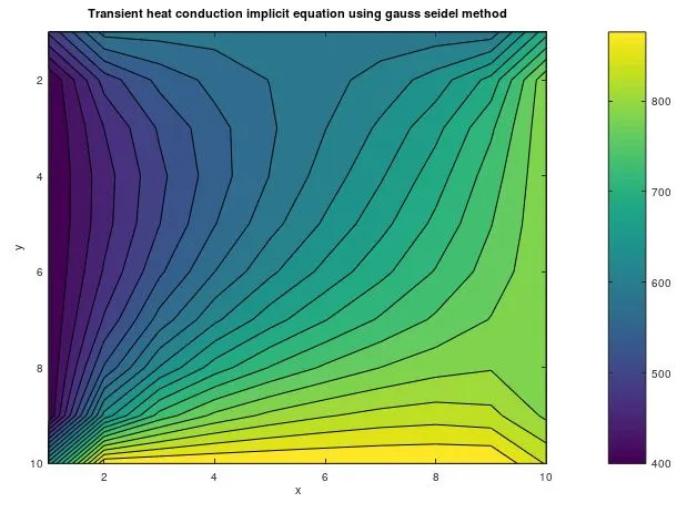

calling of function - using SOR iterative solver

function [ T ] = transient_implicit_sor(nt,error,tol,nx,ny,T,Told,alpha,T_previous_nt,term1,term2,term3)
  
Told = T;
T_previous_nt = Told ;
 
  
%time loop
  
  for k = 1:nt
  
  sor_iter = 1 ;
     while(error > tol)
     
        
        
         %space loop
         for i = 2:nx-1
       
                for j = 2:ny-1
                     
                     H = Told(i+1,j) + T(i-1,j);
                     V = Told(i,j+1) + T(i,j-1);
                     
                     T(i,j) = Told(i,j)*(1-alpha) + alpha * ((term1*T_previous_nt(i,j)) + (term2*H) + (term3*V));

                end
              
         end
  
    %updating the velocity and calculating the error
    error = max(max(abs(T - Told))) ;
    Told = T;
    
     end  
   
   %updating error value
   error = 1000;
   %calculating the residue
   error1 = max(max(abs(T - T_previous_nt)));
   %updating the tempertaure value for next time steps
   T_previous_nt = T ;
   
   %plotting the result for error with respect to nt
   figure(1);
   sor_iter = sor_iter + 1;
   title_text = sprintf('Transient heat conduction implicit equation using successive over relaxation method=%d',sor_iter);
   title(title_text)
   semilogy(k,error1,'marker','*','color','r');
   hold on;
   xlabel('number of time steps (nt)');
   ylabel('error(residue)');
   pause(0.001)
   
    
  end

    %plotting the results for temperature distribution
    figure(2);
    contourf(T,20);
    colorbar;
    set(gca,'yDIR','reverse');
    title_text = sprintf('Transient heat conduction implicit equation using successive over relaxation method');
    title(title_text)
    xlabel('x');
    ylabel('y');
    
   
endfunction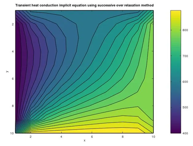

6. Results/Conclusions

• number of iteration is greater in jacobi method followed by gauss seidel and successive over relaxation method
• Jacobi iteration > Gauss Seidel iteration > SOR iteration
• This is because the jacobi method uses the same guessed value throughout its iteration for finding the converge results
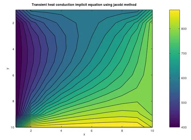
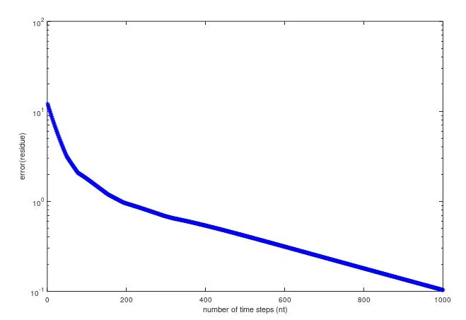
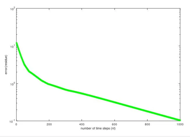
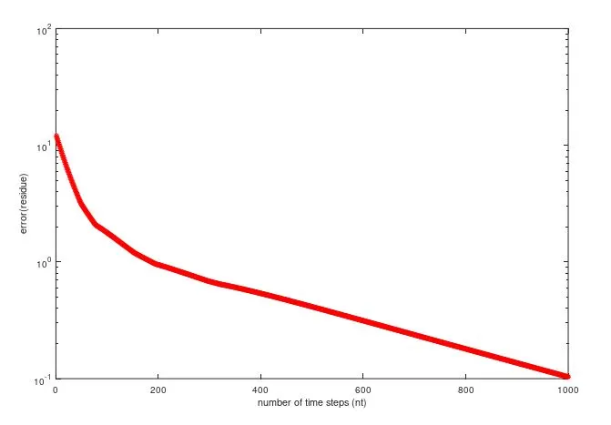
• In case of transient heat conduction implicit equation as we can see above that the error is decreasing with the time steps and our solution is reaching the steady state
• Also the time taken is more in jacobi method followed by gauss seidel and successive over relaxation method
• As we can see that the graph is same for all the cases and approach but the only difference is the time/iterations required in computing the results

Hence the steady state and transient state equation using implicit and explicit approach by use of various iterative solver is studied and computed in octave and results were analysed.