Week 9 - FVM Literature Review

In this challenge, we explore the Finite Volume Method, the need for interpolation schemes and flux limiters and how it compares with the Finite Difference Method (FDM).

FDM and FVM are effective numerical methods used to discretise and solve partial differential equations. Since partial differential equations are a staple in fluid dynamics, heat transfer and other such fields that CFD usually caters to, FDM and FVM are popular numerical methods in CFD analysis.

Despite the ease of modelling problems by discretising and solving using the finite difference approach, FVM is usally preferred in commercial solvers like OpenFOAM and ANSYS FLUENT.

This is because FDM works efficiently only for regular mesh grids. For irrregular grids, various correction factors would have to be introduced, making the effort much more cumbersome. Another way to adapt FDM for irregular grids is by the method of 'Variable Transformations'. Here, the complex geometry is adapted by linking the real world points to those in a regular grid setting by means of 'Mapping Functions'. However, devoloping these functions can also prove to be tiresome.

However, FDM finds widespread use in meteorological, seismological, and astrophysical simulations where regular grids on large scale geometries are the norm.

In FVM, instead of writing equations for a point, we write it for an elemental control volume. FVM preserves the concept of conservation.Thus, it is a more natural choice for CFD applications as most of the partial differential equations that are to solved are derived from conservation laws. A major differnce is between FDM and FVM is the use of integral forms of the conservation laws instead of the differential forms used in FDM.

Overview of the FVM approach:

1) The domain of interest is subdivided into discretised control volumes.

2) The integral form of the conservation laws are applied to these control volumes.

3) This results in a set of simplified algebraic equations that can be solved numerically.

Illustration:

The 1D heat conduction equation is to be discretised using the FVM appraoch.

`del/(delx)(alpha*(delT)/(delx))+s` ...(i)

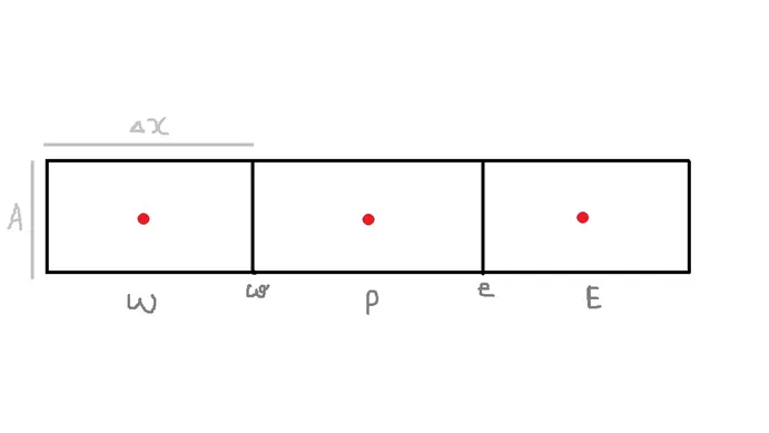
The three blocks are the discretised contol volumes. The centre of the control volume is shown in red and is a representation of the averaged values of the cell. The control volume 'P' is what is being analysed. The control volume to the left is denoted by 'W' (west) and its interface with 'P' is denoted by 'w'. Similarly, the control volume to the right is denoted by 'E' (east) and the corresponding interface is marked by 'e'. The direction along the longer dimension of the rectangle is the 'x' direction.

(Here, 'A' is the face area, the cross section is assumed to be constant throughout the domain).

on integrating equation (i) over the control volume 'P'.:

`int(del/(delx)(alpha*(delT)/(delx))+s)dv`=0 ...(ii)

here, 'dv' can be further simplified as 'Adx'.

`int(del/(delx)(alpha*(delT)/(delx))*A*dx)+intsdv`=0 ...(iii)

`alpha_eA((delT)/(delx))_e-alpha_wA((delT)/(delx))_w`+`intsdv`=0 ...(iv)

`alpha_eA(T_E-T_P)/Deltax-alpha_WA(T_P-T_W)/Deltax+barsdv=0` ...(v)

(Here, '`bars`' is an averaged value of the source term.)

On observing the eqn (v), it is seen that it can be simply represented as:

(outflux)-(influx)+heat from source=0

Thus, the form derived from FVM mathematically represents the conservational laws. This is not true for FDM. The mention of the conservational laws is lost in the final dicretised form.

The need for interpolation schemes:

Interpolation schemes are needed for transfroming the cell quantities to the face centres. In this illustration, it is needed for finding the values of temperature at the face-centres. Also, as `'alpha'`is a function of temperature, the corresponding values of `'alpha'`at the face centres can be found.

The need for grading schemes:

In this illustration, the derivatives in equation (iv) need to be calculated from the values of the temperatures (and also `'alpha'`) at the face centres. These derivatives are formulated using grading schemes. It is by using grading schemes that we can progress from equation (iv) to equation (v) which is the numerically discretised, algebraic form of the original form (as PDE) of the governing equation.

The need for Flux Limiters:

Flux limiters are an essential component in the Finite Volume Method (FVM), particularly when dealing with problems that involve shocks, discontinuities, or large gradients. The primary need for flux limiters arises from the requirement to maintain numerical stability and accuracy in the presence of such drastic changes.When high-order spatial discretization schemes are used, they can produce non-physical oscillations near discontinuities due to Gibbs phenomenon (The Gibbs phenomenon refers to the peculiar behavior of Fourier series approximations near a jump discontinuity. Specifically, it is the oscillatory behavior where the Fourier series overshoots and undershoots the actual function values around the discontinuity). These oscillations can lead to numerical instability and inaccurate solutions.The use of flux limiters ensures that the numerical solution is 'Total Variation Diminishing' (TVD), meaning that the total variation of the solution does not increase over time, which is a requirement for maintaining stability and capturing sharp changes without these unphysical numerical oscillations.