Week 9 - FVM Literature Review
Aim:FVM Literature Review;
Objective:
To write about Finite Volume Method(FVM).
To write down the major differences between FDM & FVM.
To describe the need for interpolation schemes and flux limiters in FVM by taking example of 1D linear heat conduction equation.
Theory:
Descretization is the process of dividing the domain into descrete subdomain, and the name of the subdomain depends on the method of discretization.
There are three methods to discretize the governing differential equation and make them solvable numerically.
1-Finite Difference Method
2-Finite volume method
3-Finite element method
Finite difference method is the simplest method where domain is divided into grid points called nodes and governing equations are discritized using Taylor's Series Expansion.This is not suitable when geometry is complex.
Finite element method is relatively more complicated and has to go through more rigorous formulation while discritization.It evolves from the the general principle of error minmization and does not carry the sense of conservativness.
Finite Volume Method(FVM):
This is one of the methods used to discretize partial differential equations governing the flow problem.
In this method domain is divided into logical subdomain called as control volume and it is repesented by grid volume.
Governing equations are integrated over each sub domain(control volume).Gauss Divergence theorem is used to convert volume integral into fluxes form
since these variable are stored at the centroid of the control volume, interpolation schemes are used for dependent variables to calculate fluxes at grid wall .
1-D stead state heat conduction Equation with source term-
`nabla(kdt/(dx))+S=0` eqn(1)
where S=sorce term
k=thermal conductivity
Consider there is a domain divided into three control volumes with their centroid at W,P and E .
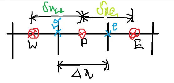
w and e are faces of the control volume.Distance btw walls of the each control volume is `Deltax` and distance of the centrod P from centrod W is `deltax_w` and fron centroid E is `deltax_e`.Dimension
Integrating equation 1 over the control volume
`int_w^ed/dx(k(dT)/dx)dx+int_w^eSdx=0`
`(k(dT)/dx)_w^e+S(w-e)=0`
if S=constant and w-e=`Deltax`
`k(dT)/dx|_e-k(dT)/dx|_w+SDeltax=0`
profile assumption is piecewise linearity between grid points
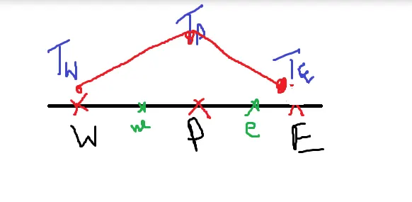
`k_e(T_E-T_P)/(deltax)_e-k_w(T_P-T_W)/(deltax)_w+SDeltax=0`
`(k_e/(deltax_e)+k_w/(deltax_w))T_P=k_e/(deltax_e)T_E+k_w/(deltax_e)T_W+Deltax`
`a_PT_P=a_ET_E+a_WT_W+b`
where `a_E=k_e/(deltax_e)`
`a_w=k_w/(deltax_w)`
`a_P=a_E+a_W`
`b=sDeltax`
Difference between FDM & FVM:
Finite difference method is the simplest method where domain is divided into grid points called nodes a while in FVM domain is divided into logical subdomain called as control volume and it is repesented by grid volume.
In FDM governing equations are discritized using Taylor's Series Expansion and solved at grid points while in FVM governing equations are integrated over each sub domain(control volume).Gauss Divergence theorem is used to convert volume integral into fluxes form.
Discretized Equation should reflect same coservativeness of variable properties as in physical problem and It is not gauranted by FDM bevacuse of truncation Taylor's series,while in FVM uses governing equationsas mass conserrvation ,momentum conservation equations which itself evolved from the guiding principle of conservativness
This is not suitable when geometry is complex while FVM can handle complex geometries as well.
Finite element method is relatively more complicated and has to go through more rigorous formulation while discritization.It evolves from the the general principle of error minmization and does not carry the sense of conservativness.
Need for interpolation schemes and flux limiters in FVM: As explained in previous section variables of governing equations are stored at the centroid of the control volume while governing equation are in integral form of fluxes so to calculate fluxes at face or get variables at the face of of control volume various interpolation scheme or profile assumption is needed.
Flux limiters are used to prevent spurious oscillations, which would otherwise appear in the solution flow field near shocks, discontinuities, or near rapid local changes in the flow field. Flux limiter schemes limit the spatial derivative to realistic values. They are used in high-resolution schemes only come into operation when sharp wave front are present.
The first order numerical schemes in space are generally too dissipative and tend to spread especially discontinuities. To improve the capture of discontinuities, we will aim to increase the accuracy of the scheme by using 2nd order scheme or equivalent, to reduce diffusivity. High order finite difference methods are less precise and dissipative, which causes numerical oscillations. In order to develop process which is high order and at the same time non-oscillating and able to capture shocks, we need to use schemes called TVD (total variation diminishing) which preserve the monotonicity and therefore increase accuracy. The method that allows to construct a scheme as a nonlinear weighting scheme between a low-order scheme and high order scheme is called flux limiter method. The flux limiter, defined as a function of smoothness controller of a numerical solution, allows limiting gradients to prevent the occurrence of oscillations.