Week 9 - FVM Literature Review

Aim:

To describe the need for the interpolation schemes in the FVM and flux limiter.

METHOD OF THE CFD:

To solve the real-world problem, the people discovery three simples schemes for the numerical solution are

• Finite Difference Method
• Finite Element Method
• Finite volume Method

Finite Difference Method:

This method solves the equation, that is divide into single points or nodes. This method involves solving the discretisation using the differencing equation.

Finite Element Method:

This method involves dividing the domain into elements of the desire. By solving the element in the system. The finite element analysis is a particular method for solving two or three-dimensional problems.

Finite Volume Method:

In the FVM Method the system to divide into an unstructured mesh which is conservative. In the algebraic form, the partial equation represents in the volume integral, which converted into the surface integral by the Gauss divergence theorem. These terms are solved as a flux in each surface. Because the flux entering the surface is identical to the adjacent surface, this is a conservative principle.

The finite volume method (FVM) is a method for representing and evaluating partial differential equations in the form of algebraic equations. In the finite volume method, volume integrals in a partial differential equation that contain a divergence term are converted to surface integrals, using the divergence theorem. These terms are then evaluated as fluxes at the surfaces of each finite volume. Because the flux entering a given volume is identical to that leaving the adjacent volume, these methods are conservative. Another advantage of the finite volume method is that it is easily formulated to allow for unstructured meshes. The method is used in many computational fluid dynamics packages. "Finite volume" refers to the small volume surrounding each node point on a mesh.

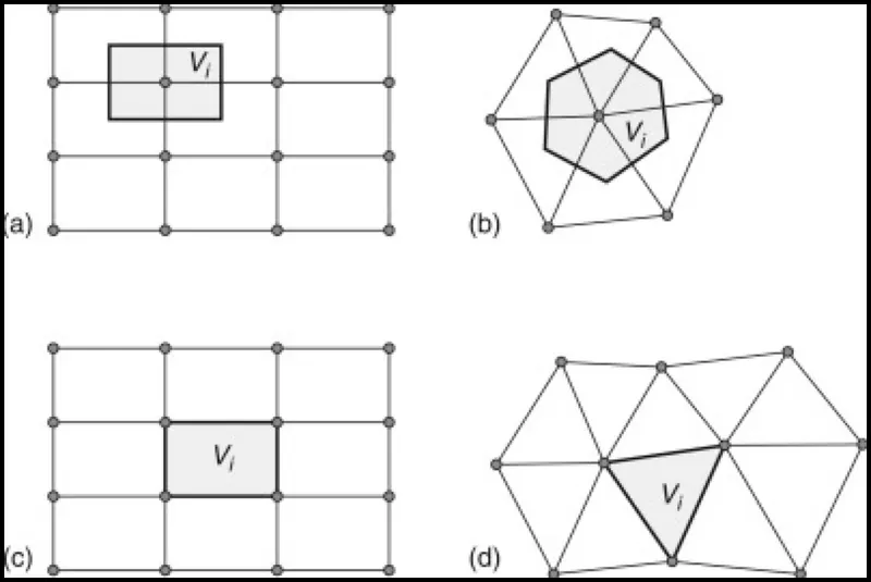
The Commercial software is based on the FVM Method because of the Unstructured mesh, Easy for solving the complex problems over the other methods.

Consider the 1D Heat Conduction Equation:

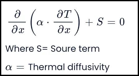
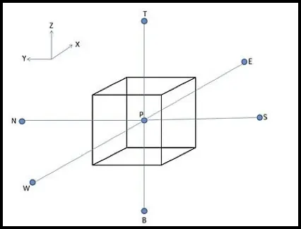
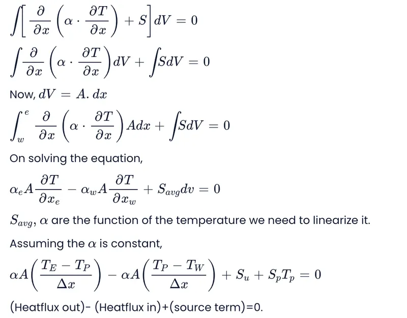
Let us consider the Control volume P and the centroid at the P as shown in the above figure. The above figure has a set of control volume with the centroids located at P, E(EAST), W(WEST), N(NORTH), S(SOUTH POINT), and the further point with the representation. The faces centre is denoted as n, e, s, and w. Come back to the Heat conduction equation, because of the 1D, it doesn't have the North and south control volume. Consider the small volume 'dv' in the Control volume P, the integral form of the equation for the small volume is given by,

Need for interpolation schemes:

To calculate the Tw and Te, Temperature at the west and east faces, we have the value at the Tp,T_E, and T_W

by interpolating the values, we can get the temperature at the east and west faces. By using them we can calculate the thermal diffusivity of the faces are α_e and α_w

There are different ways of Interpolation. Some of the ways are given by

• Upwind Interpolation scheme (UDS).
• Central Differencing Approximation. (CDS)
• Quadratic Upwind Differencing Scheme. (QUICK)
• Hybrid Interpolation Scheme. (CDS & UDS)
• Total variation Diminishing Scheme. (TVD)

Upwind Interpolation scheme (UDS):

The upwind interpolation scheme (UDS) for approximating the value of a variable at either front or black face of a control volume is given by

In this scheme we use the node in the upwind or upstream of the given node. It is generally used for convection dominated problems (i.e Pe>1).

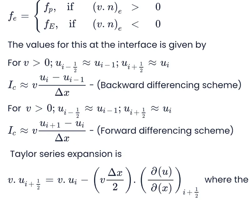
where the second term has the truncation error which resembles a diffusive Flux term.

Upwind schemes are the approximations that satisfy the boundedness unconditionally and is First order accurate in space.

Central Differencing Approximation (CDS):

(Linear Interpolation scheme)

Approximate values of the variable at the control volume (CV) face centre by the linear interpolation of the values at the two nearest computational nodes.

The value of the variable at CV face centre approximate from the values near two computational nodes. This location at 'e' on a cartesian grid, the variable value is approximated by,

The linear interpolation is equivalent to the use of the central differencing formula of the first-order derivative, and hence, this is also termed as the central differencing scheme(CDS). This scheme is the second derivative accurate and may produce an oscillatory solution.

Quadratic Upwind interpolation(QUICK)

A quadratic upwind interpolation is the three order scheme, it is derived from the polynomial fitting. It is also represented as the QUICK Interpolation.the quick interpolation on a uniform cartesian grid is given by,

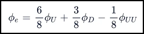
Where D, U, and UU denote the downstream, the first upstream and the second upstream node respectively. (E, P, and W or P, E, and EE) depending on the flow direction. Quick scheme is prone to oscillation because of the third order.

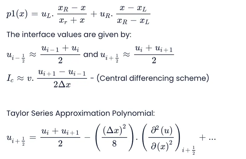
The approximation is second order precise. It is the simplest and most widely used interpolation technique for the evaluation of gradients required to measure diffusive fluxes.

Hybrid interpolation:

This companion of both the upwind and linear interpolation schemes. The cartesian grid is given by

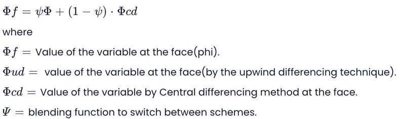
Flux limiters:

In solving the convective flow fields, it is observed that the discontinuity or shocks in results. For the High order, it is observed that the Oscillation is more and the solution became unstable due to this reason.

To obtain the highly accurate and oscillation free results we need to use the flux limiter function. The function provides the smooth region over the flow and maintains the first-order accuracy. Flux limiters are mainly used to get the total variation diminishing [TVD].

Their simple forms for 1D Equation are given by

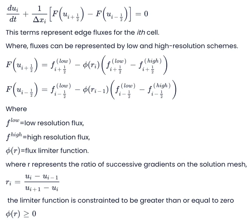
When the limiter equals to zero, the flux represents the low resolution scheme.

When the limiter equals to 1, the flux represents the high-resolution scheme.

There are many limiters having distinguished characters and are selected according to the problem. There is no particular limiter found to work well for all and it is selected by the trail and error method.

In regions with sharp temperature gradients, such as near interfaces or boundaries, numerical diffusion can occur if standard numerical schemes are used to compute the fluxes. Numerical diffusion smears out the sharp features in the temperature profile and leads to a loss of accuracy.

To mitigate this issue, flux limiters are applied to control the slope of the temperature profile and prevent excessive numerical diffusion. Flux limiters modify the gradient of temperature (i.e., the term (∂u/∂x)_P) in the flux calculation to ensure that it does not exceed certain bounds. This helps to preserve sharp temperature gradients and improve the accuracy of the solution.

The major differences between FDM and FVM:

• Basis of discretisation:
• FDM: In FDM, the domain is discretised by dividing it into a grid, and derivatives in the PDEs are approximated using finite difference formulas at the grid points.
• FVM: FVM, on the other hand, discretises the domain by dividing it into control volumes or finite volumes. The integral form of the PDEs is then applied to these control volumes to obtain algebraic equations.
• Conservation properties:
• FDM: FDM does not inherently satisfy conservation properties, such as conservation of mass, momentum, or energy. Conservation needs to be enforced separately, leading to challenges in certain applications.
• FVM: FVM inherently satisfies conservation properties because it is based on the integral form of the governing equations. The conservation laws are preserved locally for each control volume.
• Treatment of boundaries:
• FDM: FDM often uses different approaches to handle boundary conditions, such as ghost points or interpolation schemes at the boundaries.
• FVM: FVM treats boundaries naturally by incorporating the contributions of boundary fluxes to the control volume equations. This feature simplifies the implementation of boundary conditions.
• Numerical diffusion and accuracy:
• FDM: FDM tends to introduce numerical diffusion, especially in high-gradient regions, which may lead to a loss of accuracy in some cases.
• FVM: FVM is generally less diffusive than FDM, leading to better accuracy, especially for problems with steep gradients or shock waves.
• Grid structure:
• FDM: FDM typically uses structured grids, which are regular and aligned with the coordinate axes. It is more straightforward to apply FDM to regular geometries.
• FVM: FVM can handle both structured and unstructured grids, offering more flexibility for complex geometries and adaptivity.
• Conservation of discrete quantities:
• FDM: In FDM, it may not be straightforward to ensure the conservation of discrete quantities (e.g., mass, energy) across the entire domain, especially on irregular grids.
• FVM: FVM inherently guarantees the conservation of discrete quantities within each control volume, making it suitable for problems involving mass and energy balances.

Both FDM and FVM have their strengths and weaknesses, and the choice between them depends on the specific problem at hand, the geometry of the domain, and the desired accuracy and computational efficiency.