Week 4.1 - Genetic Algorithm

AIM : To write the code to calculate the global maxima of the stalagmite function and to explain the syntax for genetic algorithm(ga) in MATLAB.

Objectives :

• Write a code in MATLAB to optimise the stalagmite function and find the global maxima of the function.
• Clearly explain the concept of genetic algorithm in your own words and also explain the syntax for ga in MATLAB in your report.
• Make sure that your code gives the same output, even if it is made to run several times.
• Plot graphs for all 3 studies and for F maximum vs no. of iterations. Title and axes labels are a must, legends could be shown if necessary.

Stalagmite:

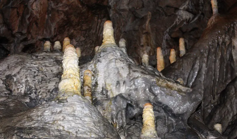
A stalagmite is a type of rock formation that rises from the floor of a cave due to the accumulation of material deposited on the floor from ceiling drippings.

Stalagmites are typically composed of calcium carbonate, but may consist of lava, mud, peat, pitch, sand, sinter, and amberat (crystallised urine of pack rats).

The corresponding formation hanging down from the ceiling of a cave is a stalactite. Mnemonics have been developed for which word refers to which type of formation;

one is that stalactite has a C for "ceiling", and stalagmite has a G for “ground", another is that, as with ants in the pants, the mites go up and the tights (tites) come down.

That is why we are using the stalagmite as the name for the program due to its shape.

Genetic Algorithm(ga):

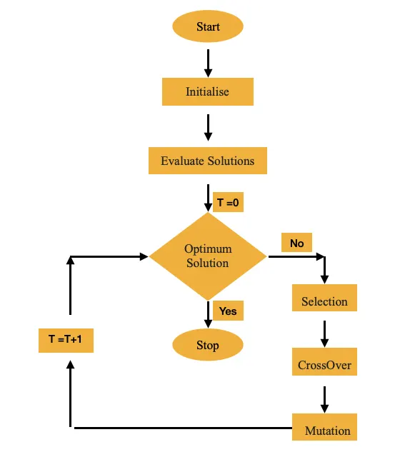
Genetic Algorithms are the heuristic search and optimisation techniques that mimic the process of natural evolution.

A genetic algorithm is an algorithm that imitates the process of natural selection.They help solve optimisation and search problems.

Genetic algorithm are part of the bigger classof evolutionary algorithms.Genetic algorithm imitates natural biological process such as inheritance , mutation , selection and crossover.

The concept of algorithm is a search technique often used compute science to find complex non-obvious solution to algorithmic optimisation and search problems.

Principle Of Natural Selection

“Select The Best, Discard The Rest”

Simple Genetic Algorithms

Selection:

• The process that determines which solutions are to be preserved and allowed to reproduce and which ones deserve to die out.
• The primary objective of the selection operator is to emphasise the good solutions and eliminate the bad solutions in a population while keeping the population size constant. “ Select the best , discards the rest”.

Functions of Selection operator

• Identify the good solutions in a population.
• Make multiple copies of good solutions.
• Eliminate the bad solutions from the population so that multiple copies of good solutions can be placed in the population.

Fitness function

• A fitness value can be assigned to evaluate the solutions.
• A fitness function value quantifies the optimality against all the other solutions.
• A fitness value is assigned to each solution depending on how close it is actually to optimal solution of the problem

Crossover operator:

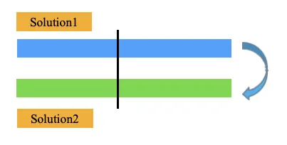
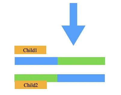
• The most popular crossover selects anyhow solutions strings randomly from the mating pool and some portion of the strings is exchanged between the strings.
• The selection point is selected randomly.
• A probability crossover is also introduced in order to give freedom to an individual solution string to determine whether the solution would go for crossover or not.

Mutation operator:

• Mutation is the occasional introduction of new features in to the solution strings of the population pool to maintain diversity in the population.
• Though crossover has the main responsibility to search for the optimal solution, mutation is also used for this purpose.

Elitism:

• Crossover and mutation may destroy the best solution of the population pool.
• Elitism is the preservation of few best solutions of the population pool.
• Elitism is defined in percentage or in number.t

Nature to computer mapping

Nature	Computer
Population	Set of solutions
Individual	Solution to a problem
Fitness	Quality of a solution
Chromosome	Encoding for a solution
Gene	Part of the encoding solution

• Selection rules select the individuals, called parents, that contribute to the population at the next generation.
• Crossover rules combine two parents to form children for the next generation.
• Mutation rules apply random changes to individual parents to form children.

Stalagmite function Equation

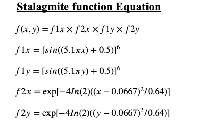
MATLAB code for Stalagmite Function

function [f] = stalagmite(V)

x=V(1);

y=V(2);

f1x = (sin((5.1*pi*x)+0.5))^6;
f1y = (sin((5.1*pi*y)+0.5))^6;
f2x = exp(-4*log(2)*(((x-0.0667)^2)/0.64));
f2y = exp(-4*log(2)*(((y-0.0667)^2)/0.64));

f = -(f1x*f1y*f2x*f2y);
end

GA Syntax :

x = ga(fun,nvars)

x = ga(fun,nvars,A,b)

x = ga(fun,nvars,A,b,Aeq,beq)

x = ga(fun,nvars,A,b,Aeq,beq,lb,ub)

x = ga(fun,nvars,A,b,Aeq,beq,lb,ub,nonlcon)

x = ga(fun,nvars,A,b,Aeq,beq,lb,ub,nonlcon,options)

x = ga(fun,nvars,A,b,Aeq,beq,lb,ub,nonlcon,intcon)

x = ga(fun,nvars,A,b,Aeq,beq,lb,ub,nonlcon,intcon,options)

x = ga(problem)

[x,fval] = ga(___)

[x,fval,exitflag,output] = ga(___)

[x,fval,exitflag,output,population,scores] = ga(___)

x = ga(fun,nvars) finds a local unconstrained minimum, x, to the objective function, fun. nvars is the dimension (number of design variables) of fun.

x = ga(fun, nvars, A,b, Aeq,beq, lb,ub, nonlcon, options)

Fun = Objective function

nvar= Number of variables ( specified as positive integer)

A,b = Linear inequality constraints ( A = Real matrix; b = Real vector)

Aeq,beq = Linear equality constraints ( A = Real matrix; b = Real vector)

lb,ub= lower bounds and upper bounds

nonlcon= Nonlinear constraints

options= Optimization options

DISCRIPTION:

x = ga(fun,nvars) finds a local unconstrained minimum, x, to the objective function, fun. nvars is the dimension (number of design variables) of fun.

x = ga(fun,nvars,A,b) finds a local minimum x to fun, subject to the linear inequalities A*x ≤ b. ga evaluates the matrix product A*x as if x is transposed (A*x\').

x = ga(fun,nvars,A,b,Aeq,beq) finds a local minimum x to fun, subject to the linear equalities Aeq*x = beq and A*x ≤ b. (Set A=[] and b=[] if no linear inequalities exist.) ga evaluates the matrix product Aeq*x as if x is transposed (Aeq*x\').

x = ga(fun,nvars,A,b,Aeq,beq,lb,ub) defines a set of lower and upper bounds on the design variables, x, so that a solution is found in the range lb ≤ x ≤ ub. (Set Aeq=[] and beq=[] if no linear equalities exist.)

x = ga(fun,nvars,A,b,Aeq,beq,lb,ub,nonlcon) subjects the minimization to the constraints defined in nonlcon. The function nonlcon accepts x and returns vectors C and Ceq, representing the nonlinear inequalities and equalities respectively. ga minimizes the fun such that C(x) ≤ 0 and Ceq(x) = 0. (Set lb=[] and ub=[] if no bounds exist.

x = ga(fun,nvars,A,b,Aeq,beq,lb,ub,nonlcon,options) minimizes with the default optimization parameters replaced by values in options. (Set nonlcon=[] if no nonlinear constraints exist.) Create options using optimoptions.

x = ga(fun,nvars,A,b,[],[],lb,ub,nonlcon,IntCon) or x = ga(fun,nvars,A,b,[],[],lb,ub,nonlcon,IntCon,options) requires that the variables listed in IntCon take integer values.

x = ga(problem) finds the minimum for problem, where problem is a structure.

[x,fval] = ga(___), for any previous input arguments, also returns fval, the value of the fitness function at x.

[x,fval,exitflag,output] = ga(___) also returns exitflag, an integer identifying the reason the algorithm terminated, and output, a structure that contains output from each generation and other information about the performance of the algorithm.

[x,fval,exitflag,output,population,scores] = ga(___) also returns a matrix population, whose rows are the final population, and a vector scores, the scores of the final population.

GA Optima MATLAB code

clear all
close all
clc
% Defining our search space
x = linspace(0,0.6,150);
y = linspace(0,0.6,150);

% Creating 2D Mesh

[xx,yy] = meshgrid(x,y);
num_case = 50;

% Evaluating the stalagmite function

for i = 1:length(xx)
    for j = 1:length(yy)

input_V(1) = xx(i,j);
input_V(2) = yy(i,j);

f(i,j) = stalagmite(input_V);
    end
end
figure(1)
surfc(xx,yy,-f);
shading interp;
title('Evaluating Stalagmite Function')
legend('Stalagmite','Global Maxima')
xlabel('x value')
ylabel('y value')

[inputs,fval] = ga(@stalagmite,2);

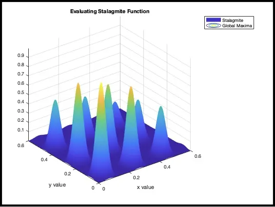
In this evaluating the optimum value of fitness function at each iteration and calculating it using the above-mentioned syntax in the intro part (which gives the inputs ie. Values of x and y at which the stalagmite function is minimum)

Then plotting it into the surf command and also providing the optimum values of the function that how it is varying.

Also using the tic and toc command to evaluate the time used for optimizing the function.

% Study 1 - Statistical behavior-Unbounded

tic
for i = 1:num_case
    [inputs,fopt(i)]=ga(@stalagmite,2);
  
    xopt(i) = inputs(1);
    yopt(i) = inputs(2);
end
study1_time = toc

figure(2)
subplot(2,1,1)
hold on
surfc(x,y,-f)
shading interp
plot3(xopt,yopt,-fopt,'marker','o','MarkerSize',5,'MarkerFaceColor','r')
title('Statistical Behaviour of Unbounded Inputs')
legend('Stalagmite','Global Maxima')
xlabel('x value')
ylabel('y value')
subplot(2,1,2)
plot(fopt)
xlabel('Iterations')
ylabel('Function maximum')

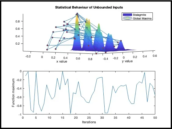
From the figure as shown above it is clear that the results are not that much accurate and giving a lot of variation in optimizing the function.

% Study 2 - Statistical behavior -with upper and lower bounds
tic
for z = 1:num_case
    [inputs,fopt(z)]=ga(@stalagmite,2,[],[],[],[],[0;0],[0.6;0.6]);
    % defines a set of lower and upper,bounds on the design variables
    xopt(z) = inputs(1);
    yopt(z) = inputs(2);
end
study2_time = toc

figure(3)
subplot(2,1,1)
hold on
surfc(x,y,-f)
shading interp
plot3(xopt,yopt,-fopt,'marker','o','MarkerSize',5,'MarkerFaceColor','r')
title('Statistical Behaviour of Bounded Inputs')
legend('Stalagmite','Global Maxima')
xlabel('x value')
ylabel('y value')
subplot(2,1,2)
plot(fopt)
xlabel('Iterations')
ylabel('Function maximum')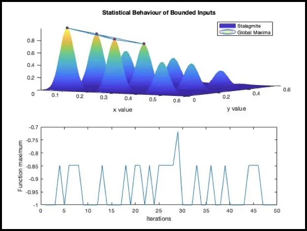

It is clearly seen from the above that after providing the boundary limits the variation in the optimum value of the function has reduced.

% Study 3 - Statistical behavior -Bounded GA study with population size
options = optimoptions('ga');
options = optimoptions(options,'PopulationSize',270);
tic
for z = 1:num_case
    [inputs,fopt(z)]=ga(@stalagmite,2,[],[],[],[],[0;0],[0.6;0.6],[],[],options);
    % defines a set of lower and upper,bounds on the design variables
    xopt(z) = inputs(1);
    yopt(z) = inputs(2);
end
study3_time = toc

figure(4)
subplot(2,1,1)
hold on
surfc(x,y,-f)
shading interp
plot3(xopt,yopt,-fopt,'marker','o','MarkerSize',5,'MarkerFaceColor','r')
title('Statistical Behaviour of Bounded Inputs & Population Size')
legend('Stalagmite','Global Maxima')
xlabel('x value')
ylabel('y value')
subplot(2,1,2)
plot(fopt)
xlabel('Iterations')
ylabel('Function maximum')

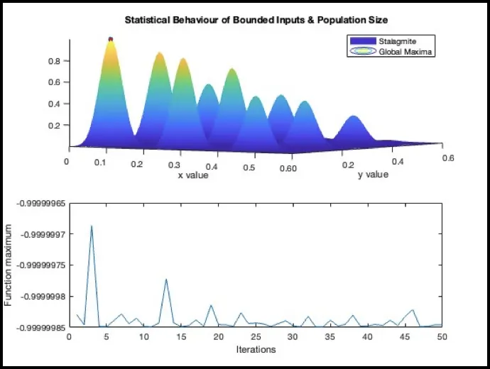
In this study using the ‘optimoptions’ command to increase the size of population.

The benefit of that will be it will be working on the large set of numbers and which will be led to increase the possibilities of finding the better fitness of the function.

It is giving single point solution.

Multi-objective optimization

Two objectives are:

• Minimise weight
• Minimise deflection

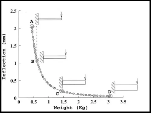
• More than one objectives
• Objectives are conflicting in nature
• Dealing with two search space

• Decision variable space
• Objective space

• Unique mapping between the objectives and often the mapping is non-linear.
• Properties of the two search space are not similar.
• Proximity of two solutions in one search space does not mean a proximity in other search space.

References:

https://en.wikipedia.org/wiki/Genetic_algorithm

https://in.mathworks.com/help/gads/ga.html

https://www.iitg.ac.in/rkbc/CE602/CE602/Genetic%20Algorithms.pdf