Week 3 - Solving second order ODEs

Aim:-

To solve an ordinary differential equation (ODE) and use the calculated information to animate the motion of the pendulum via MatLab.

Introduction:-

Pendulums have many applications and were utilized often before the digital age. They are used in clocks and metronomes due to the regularity of their period, in wrecking balls and playground swings, due to their simple way of building up and keeping energy.

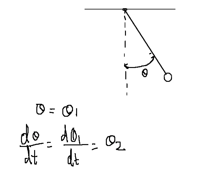
A simple pendulum consists of a point mass suspended on a string or wire that has negligible mass. If the pendulum weight or bob is pulled to a relatively small angle from the vertical and let go, it will swing back and forth at a regular period and frequency. Figure 1 shows a simple pendulum model

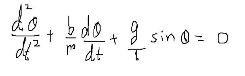
Newtons second law is a quantitative description of the changes that force can produce on the motion of a body. It states that the time rate of change of momentum of a body is equal in both magnitude and direction to the force imposed on it.

F = mass x acceleration
And above second oder equation

Small change in angular displacement theta is equal to theta1 After

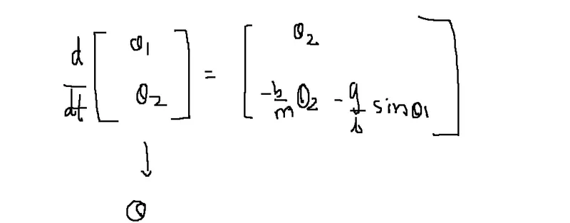
dtheta1_dt = theta2

Simplify above equation in to first oder equation.

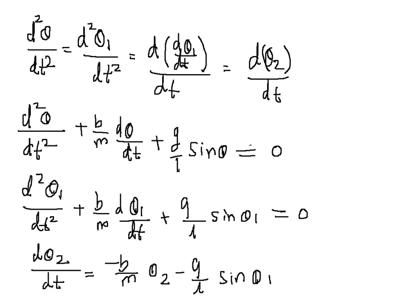
Above solution in matrix format displacement.

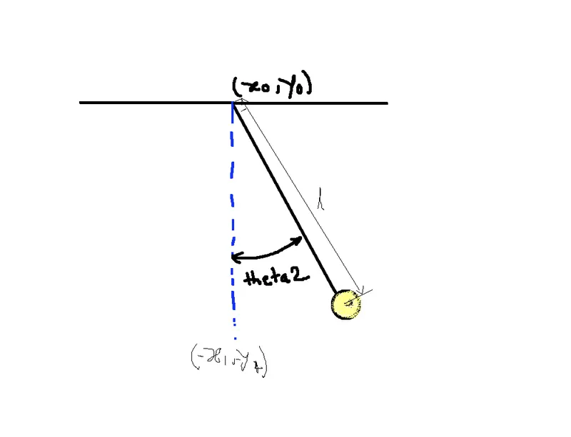
Confusion in horizontal and vertical motion .

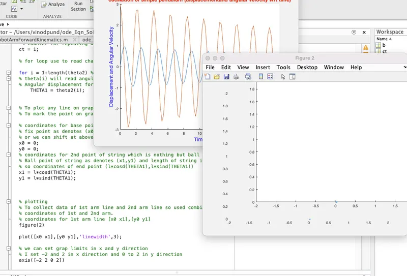
x1 = l*cosd(THETA1);

y1 = l*sind(THETA1);

Which creat horizontal line.

Our requirement is vertical pendulum oscillation and most

important we have angular displacement so second ball point

become

x1 = l*sin(THETA1);

y1 = l*cos(THETA1);

Negative sign before x1 and y1 point shows downward direction of string.

To create movie file and animation robotic code help me lot to understand and create animation video.

ODE Function

function[dtheta_dt] = ode_func(t,theta,b,g,l,m)

%t = time for oscillation

% theta = angular displacement

%g = gravity in m/s2,

%l = length of the pendulum in m,

%m = mass of the ball in kg,

%b=damping coefficient.

% simplify condition that every angular displacement

theta1 = theta(1); % first angular displacement

theta2 = theta(2); % second angular displacement

dtheta1_dt = theta2; % first angular displacement change wrt time is nothing but second angular displacement

dtheta2_dt = -(b/m)*theta2-(g/l)*sin(theta1); % second order equation is converted in to first oder equation

dtheta_dt = [dtheta1_dt; dtheta2_dt];% we are calculating every changes in angular displacment there will be change in velocity w. r. t. time

end

MATLAB main code

clear all

close all

clc

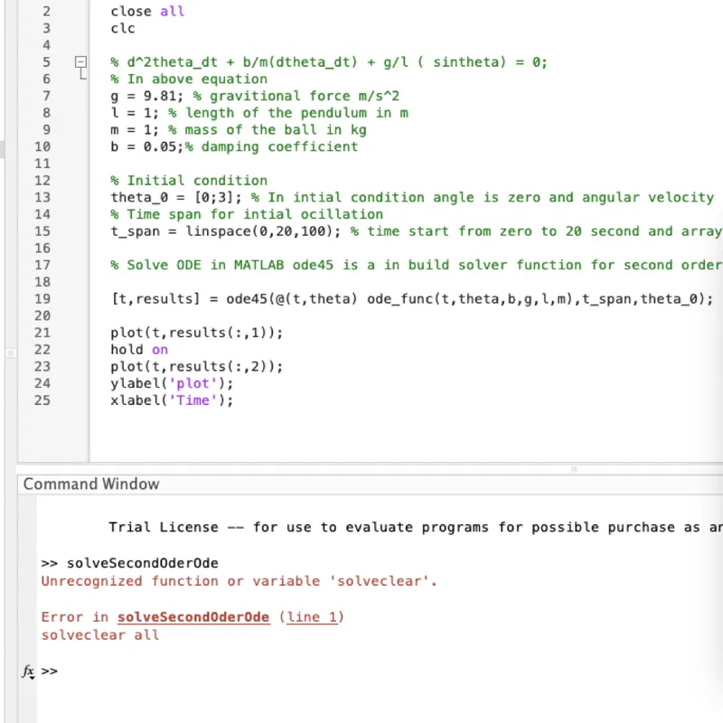
% d^2theta_dt + b/m(dtheta_dt) + g/l ( sintheta) = 0;

% In above equation

g = 9.81; % gravitional force m/s^2

l = 1; % length of the pendulum in m

m = 1; % mass of the ball in kg

b = 0.05;% damping coefficient

% Initial condition

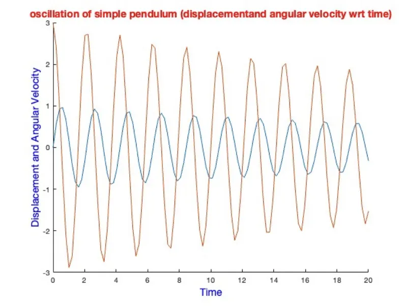
theta_0 = [0;3]; % In intial condition angle is zero and angular velocity that means 3 rad/s

% Time span for intial ocillation

t_span = linspace(0,20,100); % time start from zero to 20 second and array of interval 100

% Solve ODE in MATLAB ode45 is a in build solver function for second order

[t,results] = ode45(@(t,theta) ode_func(t,theta,b,g,l,m),t_span,theta_0);

figure(1)

hold on

plot(t,results(:,1)); % first column represents the angular displacement in rad

plot(t,results(:,2)); % seconf column represents the angular velocity in rad/s

title('oscillation of simple pendulum (displacementand angular velocity wrt time)','FontSize',14,'color','r');

xlabel('Time','FontSize',14,'Color','b');

ylabel('Displacement and Angular Velocity','FontSize',14,'Color','b');

% To create animation so extract every angular displacement of simple pendulum ball wrt time

% theta2 angular displacement of ball interval of 100 every degree angular movement

theta2 = results(:,1);

% counter for repeating and adding loop every movement till complete all assigned change

ct = 1;

% for loop use to read changes in both string and ball to plot every changes

for i = 1:length(theta2) % i is vector operator for ball with string

% theta(i) will read angular change from 0 to 20 with interval of 100

% Angular displacement for every position as per input and store in THETA1

THETA1 = theta2(i);

% To plot any line on grap require points start point and end point

% To mark the point on graph , it requires coordinates of x and y direction

% coordinates for base point of string

% fix point as denotes (x0,y0) so coordinates of start point (0,0) we can assume

% or we can shift at above base level also per requirement

x0 = 0;

y0 = 0;

% coordinates for 2nd point of string which is nothing but ball end

% Ball point of string as denotes (x1,y1) and length of string is l,

% so coordinates of end point (l*cosd(THETA1),l*sind(THETA1))

x1 = l*sin(THETA1);

y1 = l*cos(THETA1);

% plotting horizontal support line curve on plot

% To collect data of 1stline and 2nd ball so used combine

% coordinates of 1st and 2nd point.

% coordinates for 1st arm line [x0 x1],[y0 y1]

figure(2)

plot([-1 1],[0 0],'color','b','linewidth',3);% It creates fixed horizontal line support

hold on % This syntax hold on hold line grap in same plot

plot([x0 -x1],[y0 -y1],'color','r','linewidth',3);% (x0,y0) fixed position and

% (x1,y1) this gives us angular displacement varies with incremental of

% theta2 in put data from results(:,1) extract.Negative sign for x1 y1 help

% to show downward line for string

hold on

plot(-x1,-y1,"Marker","o",'MarkerSize',20,'MarkerFaceColor','y'); % This syntax help to create ball on (x1,y1) point

title('Simple Pendulum Oscillation','FontSize',18,'color','b');

hold off

% we can set grap limits in x and y direction

% I set -2 and 2 in x direction and 0 to 2 in y direction

axis([-2 2 -2 2]);

% To control processing speed of code it require pause in second

pause(0.1);

% To capture every changes in grap at every change in points or line

% movements and capture every count so extracted count as M(ct)

% fig = gcf, fig = gcf returns the current figure handle.

% If a figure does not exist, then gcf creates a figure and returns its handle.

% getframe(gcf) will extract fig of plotting and store in M(ct)

M(ct) = getframe(gcf);

% counter for increment every stage forward so ct + 1

ct = ct + 1;

end % end of i loop

% movie(M) plays the movie frames in array M once.

% To create a movie frame from the current figure

movie(M);

% To create video file syntax; v = VideoWriter(filename,profile)

% additionally applies a set of properties tailored to a specific file

% format (such as 'MPEG-4' or 'Uncompressed AVI').

V = VideoWriter('simple_pendulum.avi','Uncompressed AVI');

% Open file for writing video data

open(V);

% Write video data to file

writeVideo(V,M);

% Close file after writing video data

close(V);

https://www.youtube.com/watch?v=nbOg1ZKSxDk