Week 9 - FVM Literature Review

AIM: To define

1. Finite Volume Method(FVM).
2. The major Differences between FDM & FVM.
3. Describe the need for interpolation schemes and flux limiters in FVM.

Discretization: The Numerical Solution of Differential Equations cannot produce a continuous distribution of the variables over the solution domain. Discretization is the method used to produce a set of discrete values at a number of nodes that cover the solution domain.

Methods of Descritization:

1. Finite Difference Method(FDA).
2. Finite Element Method(FEA).
3. Finite Volume Method(FVM).

1. Finite Difference Method:

In numerical analysis FDM are a class of numerical techniques for solving Differential Equations by approximating derivatives with finite differences. FDM converts Ordinary Differential Equations(ODE) or Partial Differential Equations(PDE) which maybe nonlinear into system of linear equations.

2. Finite Element Method:

The FEM is a particular numerical method for solving partial differential equations in two or three space variables (i.e., some boundary value problems). To solve a problem, the FEM subdivides a large system into smaller, simpler parts that are called finite elements. This is achieved by a particular space discretization in the space dimensions, which is implemented by the construction of a mesh of the object: the numerical domain for the solution, which has a finite number of points.

3. Finite Volume Method:

The finite volume method (FVM) is a method for representing and evaluating partial differential equations in the form of algebraic equations. In the finite volume method, volume integrals in a partial differential equation that contain a divergence term are converted to surface integrals, using the divergence theorem. These terms are then evaluated as fluxes at the surfaces of each finite volume. Because the flux entering a given volume is identical to that leaving the adjacent volume, these methods are conservative. Another advantage of the finite volume method is that it is easily formulated to allow for unstructured meshes.

Finite volume methods can be compared and contrasted with the finite difference methods, which approximate derivatives using nodal values, or finite element methods, which create local approximations of a solution using local data, and construct a global approximation by stitching them together. In contrast a finite volume method evaluates exact expressions for the average value of the solution over some volume, and uses this data to construct approximations of the solution within cells.

FDM vs FVM:

FDM

• Mostly for defined geometries which could be represented by structured grids.
• This method is a subset of finite element method as it works mainly for structured spatial discretization. Which means, the problems solved by finite difference method could be solved using finite element method, but the converse is not necessarily true.
• One of the deviations in the case of FDM would come from approximating the higher order terms in Taylor’s series which is used to linearize the PDE. This is called as truncation error.
• Other important differentiating factor of FDM compared to FEM and FVM is that it is based on the differential form of governing equations. FEM and FVM are based on the integral form or weak formulation.

FVM:

• The properties are calculated for every cell instead of a node
• Based on the integral form of conservation laws and can handle discontinuities in solutions. In simple terms, what comes in, must go out.
• FVM approximates the value of the integral on the reference cell
• Efficient in solving fluid flow problems
• Like FEM, lot of established and theoretically proven subroutines are in place for FVM which can be directly implemented in your code.

Interpolation Schemes:

Interpolation schemes are used to transform cell-centre quantities to face centres. The operation is used in many of the finite volume calculations.

e.g. for the calculation of gradient, divergence, and Laplacian terms

• The interpolation scheme can calculate the appropriate derivatives required for the calculus equations.
• Interpolation equations depend on the neighboring cells.

The following are some Interpolation schemes which are widely used in CFD.

1. Upwind Interpolation scheme.

2. QUICK scheme(Quadratic Upstream Interpolation for Convective Kinematics).

1. Upwind Interpolation Scheme:

Upwind schemes denote a class of numerical discretization methods for solving hyperbolic partial differential equations. Upwind schemes use an adaptive or solution-sensitive finite difference stencil to numerically simulate the direction of propagation of information in a flow field. The upwind schemes attempt to discretize hyperbolic partial differential equations by using differencing biased in the direction determined by the sign of the characteristic speeds.

1st Order Upwind scheme:

consider 1D linear advection equation:

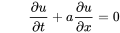
The equation describes a wave propagating along the x-axis with a velocity a. This equation is also a mathematical model for one-dimensional linear advection. Consider a typical grid point i in the domain. In a one-dimensional domain, there are only two directions associated with point i – left (towards negative infinity) and right (towards positive infinity). If a is positive, the travelling wave solution of the equation above propagates towards the right, the left side of i is called upwind side and the right side is the downwind side. Similarly, if a is negative the travelling wave solution propagates towards the left, the left side is called downwind side and right side is the upwind side. If the finite difference scheme for the spatial derivative contains more points in the upwind side, the scheme is called an upwind-biased.

The following are the 1st order upwind scheme

which is a general way of writing any upwind-type schemes.

and the Upwind scheme is stable if it satisfies Courant–Friedrichs–Lewy condition which is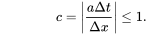

2nd Order Upwind scheme:

The spatial accuracy of the first-order upwind scheme can be improved by including 3 data points instead of just 2, which offers a more accurate finite difference stencil for the approximation of spatial derivative. For the second-order upwind scheme,

u_x becomes the 3-point backward difference in equation (3) and is defined as

and is the 3-point forward difference, defined as

This scheme is less diffusive compared to the first-order accurate scheme and is called linear upwind differencing (LUD) scheme.

3rd Order scheme:

For the third-order upwind scheme, in equation (3) which is defined as

and is defined as

This scheme is less diffusive compared to the second-order accurate scheme and it is known to introduce slight dispersive errors in the region where the gradient is high.

2. QUICK scheme(Quadratic Upstream Interpolation for Convective Kinematics):

This is a higher-order differencing scheme that considers a three-point upstream weighted quadratic interpolation for the cell face values.

• In order to find the cell face value a quadratic function passing through two bracketing or surrounding nodes and one node on the upstream side must be used. In central differencing scheme and second order upwind scheme the first order derivative is included and the second order derivative is ignored.
• These schemes are therefore considered second order accurate where as QUICK does take the second order derivative into account, but ignores the third order derivative hence this is considered third order accurate.
• This scheme is used to solve convection–diffusion equations using second order central difference for the diffusion term and for the convection term the scheme is third order accurate in space and first order accurate in time. QUICK is most appropriate for steady flow or quasi-steady highly convective elliptic flow.

Quadratic Interpolation for QUICK scheme:

For the one-dimensional domain the Φ value at a control volume face is approximated using three-point quadratic function passing through the two bracketing or surrounding nodes and one other node on upstream side. In order to calculate the value of the property at the face, we should have three nodes i.e. two bracketing or surrounding nodes and one upstream node as shown.

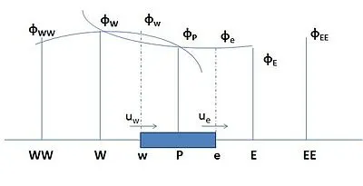
• Φw when uw > 0 and ue > 0 a quadratic fit through WW, W and P is used,
• Φe when uw > 0 and ue > 0 a quadratic fit through W, P and E is used,
• Φw when uw < 0 and ue < 0 values of W, P and E are used,
• Φe when uw < 0 and ue < 0 values of P, E and EE are used.

When the flow is in positive direction the values of the velocities u_w & u_e > 0.

When the flow is in negative direction the values of the velocities u_w & u_e < 0.

FLUX Limiters:

• Flux limiters are used in high resolution numerical schemes used to solve problems fluid dynamics, described by partial differential equations (PDE's).
• Flux limiters are also referred to as slope limiters because they both have the same mathematical form, and both have the effect of limiting the solution gradient near shocks or discontinuities. In general, the term flux limiter is used when the limiter acts on system fluxes, and slope limiter is used when the limiter acts on system states (like pressure, velocity etc.).
• The main idea behind the construction of flux limiter schemes is to limit the spatial derivatives to realistic values – for scientific and engineering problems this usually means physically realisable and meaningful values.
• For smoothly changing waves, the flux limiters do not operate and the spatial derivatives can be represented by higher order approximations without introducing spurious oscillations.

Consider 1D semi-discrete scheme:

where

and

represent edge fluxes for the ith cell.

If these edge fluxes can be represented by low and high resolution schemes, then a flux limiter can switch between these schemes depending upon the gradients close to the particular cell, as follows,

,

,

low resolution flux,

high resolution flux,

flux limiter function,

and r represents the ratio of successive gradients on the solution mesh, i.e.,

The limiter function is constrained to be greater than or equal to zero

• when the limiter is equal to zero (sharp gradient, opposite slopes or zero gradient), the flux is represented by a low resolution scheme.
• when the limiter is equal to 1 (smooth solution), it is represented by a high resolution scheme.