Week 7 - Simulation of a 1D Super-sonic nozzle flow simulation using Macormack Method

AIM: To simulate the isentropic flow through a quasi 1D subsonic-supersonic nozzle by deriving the conservation and non-conservation forms of the governing equations by solving the MacCormack's technique and determine the steady-state temperature distribution for the flow-field variables and investigate the difference between the two forms of governing equations by comparing their solutions.

Solution:

Consider a steady, isentropic flow through a convergent-divergent nozzle as shown in below fig.

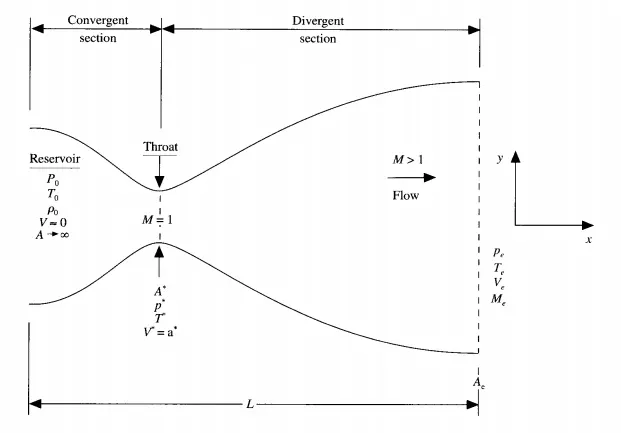
The flow at the inlet to the nozzle comes from reservoir where the cross-sectional area is large and hence the velocity will be low.

The flow is locally subsonic in the convergent part(M<1) of nozzle, sonic at the throat(M=1) and supersonic at the divergent (M>1). The sonic flow at the throat having the velocity which is equal to the local speed of sound.

Non-Conservative and Conservative form of Governing Equations:

The assumption of flow properties varies along the length of x direction and remains uniform across other direction is known as 1D Quasi Flow.

Methodology:

1.Mesh

2.Discretization

3.Solve i. Initial Conditions ii. Boundary Conditions

Methodology:

we will set up three steps of equations.

1. The governing equations flow will be couched in terms of Partial Differential Equations suitable for the time marching solution of Quasi 1D flow.

2. The Finite difference expressions pertaining to MacCormack's Method as applied to this problem will be setup. The steps in MacCormack's method are:

(a) Predictor Step = which uses Forward differencing

(b) Corrector Step = which uses Backward differencing

3. Calculation of the time steps and the treatment of Boundary Conditions.

Non-Conservative Form:

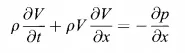
1. Momentum Equation	Dimensional	Non-Dimensional
2. Continuity Equation
3. Energy Equation

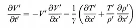
Predictor Step: Uses forward differencing

1.

2.

3.

Corrector Step: Uses backward differencing

1.

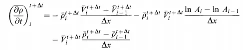
2.

3.

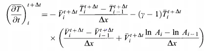
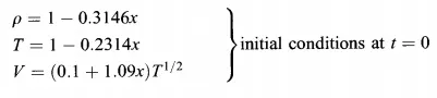
 Calculation of Time step = delta*t = C*((delta*t)/(a+v))

Initial Conditions:

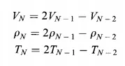
Boundary Conditions:

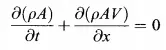
Conservative Form:

1. Momentum Equation	Dimensional	Non-Dimensional
2. Continuity Equation
3. Energy Equation

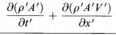
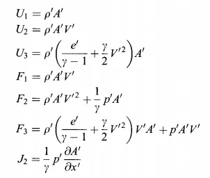
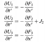
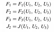
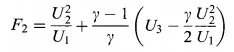
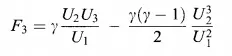
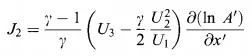
Flux Calculation:

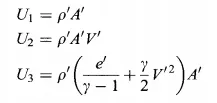
Initial Conditions:

Boundary Conditions:

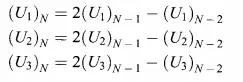
MATLAB CODE:

Main Code:

%  Simulation of a 1D Super-sonic nozzle flow simulation using Macormack Method

clear all
close all
clc

% Inputs
n = 61
x = linspace(0,3,n);
dx = x(2) - x(1);
gamma = 1.4;
nt = 1400; % Time steps


% Non-Conservative Form of Solving
[rho,v,t,m_nc,M_nc,p_nc,rho_throat_nc,v_throat_nc,t_throat_nc,p_throat_nc,M_throat_nc]=non_conservative1(n,x,dx,gamma);

% Conservative Form of Solving
[rho_c,v_c,t_c,k,m_c,M_c,p_c,rho_throat_c,v_throat_c,M_throat_c,t_throat_c,p_throat_c]=Conservative_form1(n,x,dx,gamma);

% Plotting Comparison of Parameters with Length
figure(5)
subplot(4,1,1)
plot(x,t,'*--b')
hold on
plot(x,t_c,'b')
xlabel('Length')
ylabel('Temperature')
title('Distribution of Parameters with respect to Length')
legend('* Non-Conservative','- Conservative')
grid on

subplot(4,1,2)
plot(x,rho,'*--g')
hold on
plot(x,rho_c,'g')
xlabel('Length')
ylabel('Density')
grid on

subplot(4,1,3)
plot(x,M_nc,'*--r')
hold on
plot(x,M_c,'r')
xlabel('Length')
ylabel('Mach Number')
grid on

subplot(4,1,4)
plot(x,p_nc,'*--k')
hold on
plot(x,p_c,'k')
xlabel('Length')
ylabel('Pressure')
grid on


% Plotting of Throat Values
% Plotting Comparison of Parameters at throat
figure(6)
subplot(4,1,1)
plot(t_throat_nc,'b')
hold on
plot(t_throat_c,'m')
xlabel('Length')
ylabel('Temperature')
title('Distribution of Parameters with at throat')
legend('Non-Conservative','Conservative')
grid on

subplot(4,1,2)
plot(rho_throat_nc,'g')
hold on
plot(rho_throat_c,'m')
xlabel('Length')
ylabel('Density')
legend('Non-Conservative','Conservative')
grid on

subplot(4,1,3)
plot(M_throat_nc,'r')
hold on
plot(M_throat_c,'m')
xlabel('Length')
ylabel('Mach Number')
legend('Non-Conservative','Conservative')
grid on

subplot(4,1,4)
plot(p_throat_nc,'k')
hold on
plot(p_throat_c,'m')
xlabel('Length')
ylabel('Pressure')
legend('Non-Conservative','Conservative')
grid on


% Plotting of Non-Conservative and Conservative Mass Flow
figure(7)
plot(x,m_nc,'*--b')
hold on
plot(x,m_c,'*--r')
xlabel('Length of Nozzle')
ylabel('Mass Flow')
grid on
legend('Non-Conservative Mass Flow rate','Conservative Mass Flow')

Code for Non_Conservative Form:

function[rho,v,t,m_nc,M_nc,p_nc,rho_throat_nc,v_throat_nc,t_throat_nc,p_throat_nc,M_throat_nc]=non_conservative1(n,x,dx,gamma)

% Inputs
%n = 31;
x = linspace(0,3,n);
dx = x(2)-x(1);
gamma = 1.4;

% Calculate Initial profiles
rho = 1-0.3146*x;               % rho = density profile
t = 1-0.2314*x;                 % t = temperature profile
v = (0.1+1.09*x).*(t.^(0.5));   % v = velocity profile

% Area
a = (1+2.2*(x-1.5).^2);

% Throat
throat = find(a==1);

% Time steps
nt = 1400;
c = 0.5;
dt = min(c*(dx./(sqrt(t)+v)));

% Outer time loop
for k = 1:nt
    
    dt = min((c*dx./(sqrt(t)+v)));
    
    rho_old = rho;
    v_old = v;
    t_old = t;
    
    % Predictor Method
    % Predictor method uses Forward differencing
    for j = 2:n-1
        
        dvdx = (v(j+1)-v(j))/dx;
        drhodx = (rho(j+1)-rho(j))/dx;
        dtdx = (t(j+1)-t(j))/dx;
        dlogadx = (log(a(j+1))-log(a(j)))/dx;
        
        % Continuity Equation
        drhodt_p(j) = -rho(j)*dvdx-rho(j)*v(j)*dlogadx-v(j)*drhodx;
        
        % Momentum Equation
        dvdt_p(j) = -v(j)*dvdx - (1/gamma)*(dtdx + (t(j)/(rho(j))*drhodx));
        
        % Energy Equation
        dtdt_p(j) = -v(j)*dtdx-(gamma-1)*t(j)*(dvdx+v(j)*dlogadx);
        
        % Solution update
        v(j) = v(j) + dvdt_p(j)*dt;
        rho(j) = rho(j) + drhodt_p(j)*dt;
        t(j) = t(j) + dtdt_p(j)*dt;
      end
    
     % Corrector Method
     % Corrector Method uses Backward Differencing 
      for j = 2:n-1
          
          dvdx = (v(j)-v(j-1))/dx;
          drhodx = (rho(j)-rho(j-1))/dx;
          dtdx = (t(j)-t(j-1))/dx;
          dlogadx = (log(a(j))-log(a(j-1)))/dx;
          
          % Continuity Equation
          drhodt_c(j) = -rho(j)*dvdx - rho(j)*v(j)*dlogadx - v(j)*drhodx;
          
          % Momentum Equation
          dvdt_c(j) = -v(j)*dvdx - (1/gamma)*(dtdx + (t(j)/(rho(j))*drhodx));
          
          % Energy Equation
          dtdt_c(j) = -v(j)*dtdx - (gamma-1)*t(j)*(dvdx + v(j)*dlogadx);    
      end
    
      % Average time derivative
      drhodt = 0.5*(drhodt_p + drhodt_c);
      dvdt = 0.5*(dvdt_p + dvdt_c);
      dtdt = 0.5*(dtdt_p + dtdt_c);
      
      % Final Solution update  
      for i = 2:n-1
          rho(i) = rho_old(i) + drhodt(i)*dt;
          v(i) = v_old(i) + dvdt(i)*dt;
          t(i) = t_old(i) + dtdt(i)*dt;
      end

      % Apply the Boundary conditions
      % Inlet
      rho(1) = 1;
      v(1) = 2*v(2) - v(3);
      t(1) = 1;
          
      % Outlet
      v(n) = 2*v(n-1) - v(n-2);
      rho(n) = 2*rho(n-1) - rho(n-2);
      t(n) = 2*t(n-1) - t(n-2);
        
    
      m_nc = rho.*v.*a;  % Mass Flow Rate
      p_nc = rho.*t;     % Pressure
      M_nc = v./sqrt(t); % Mach number
      
      % Throat Value Calculation
      rho_throat_nc(k) = rho(throat);
      v_throat_nc(k) = v(throat);
      p_throat_nc(k) = p_nc(throat);
      t_throat_nc(k) = t(throat);
      M_throat_nc(k) = M_nc(throat);
      
      % Plotting of Mass flow at different time step
        figure(1)
        hold on
            if k==50
                plot(x,m_nc,'b')
              else if k==100
                plot(x,m_nc,'g')
              else if k==200
                plot(x,m_nc,'r')
              else if k==400
                plot(x,m_nc,'k')
              else if k==600
                plot(x,m_nc,'y')
              
             xlabel('Non-Dimensional Nozzle Length')
                    ylabel('Non-Dimensional Mass Flow Rate')
                    legend('50dt','100dt','200dt','400dt','600dt')
                    title('Non-Conservative Mass Flow at differnt Time Steps')
                    grid on
                  end
                end
              end
            end
          end
      end   
      % Plotting of parameters with respect to length  
      figure(2)
        subplot(4,1,1)
        plot(x,M_nc)
        xlabel('Length of Nozzle')
        ylabel('Mach Number')
        title(sprintf('Time step = %d',k))
        pause(0.03)
        grid on
        
        subplot(4,1,2)
        plot(x,p_nc)
        xlabel('Length of Nozzle')
        ylabel('Pressure')
        grid on
        
        subplot(4,1,3)
        plot(x,rho)
        xlabel('Length of Nozzle')
        ylabel('Density')
        grid on
        
        subplot(4,1,4)
        plot(x,t)
        xlabel('Length of Nozzle')
        ylabel('Temperature')
        grid on
        
      end

Results for Non-Conservative:

1. The following is the mass flow for different time steps at n=31.

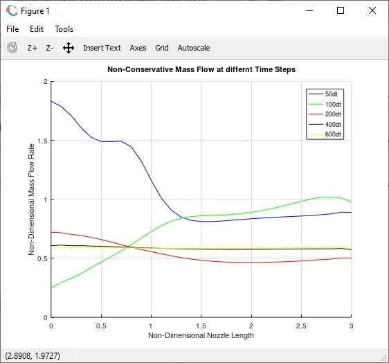
The mass flow at time step 50 is high cause of the entry of the fluid in its initial stages. The mass flow reduced slowly and attained steady value at time step 400.

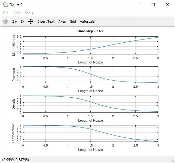
2. Mach number, Pressure, Density, Temperature distribution through Nozzle.

Code for Conservative Form:

function[rho_c,v_c,t_c,k,m_c,M_c,p_c,rho_throat_c,v_throat_c,M_throat_c,t_throat_c,p_throat_c]=Conservative_form1(n,x,dx,gamma)

%Inputs
%n = 31;
x = linspace(0,3,n);
dx = x(2)-x(1);
gamma = 1.4;

% Calculate Initial profiles
    for j=1:n
        if (x(j)>=0 && x(j)<=0.5)
            rho_c(j)=1;
            t_c(j)=1;
        elseif (x(j)>=0.5 && x(j)<=1.5)
            rho_c(j)=1-0.366*(x(j)-0.5);
            t_c(j)=1-0.167*(x(j)-0.5);
        elseif (x(j)>=1.5 && x(j)<=3.5)
            rho_c(j)=0.634-0.3879*(x(j)-1.5);
            t_c(j) = 0.833-0.3507*(x(j)-1.5);
        end
    end         
    % Area
    a = 1 + 2.2*(x-1.5).^2;
    
    % Throat
    throat = find(a==1);
           
    % Velocity
    v_c = 0.59./(rho_c.*a);
                   
    % Pressure
    p_c = rho_c.*t_c;
            
    % Initial
    U1 = rho_c.*a;
    U2 = U1.*v_c;
    U3 = U1.*(t_c./(gamma-1)+(gamma/2).*(v_c.^2));
    
    % Time loop
    nt = 1400;
    C = 0.5;
             
    % Outer Time Loop
    for k = 1:nt
        
        dt = min(C.*(dx./((t_c.^0.5) + v_c)));
        
        U1_old = U1;
        U2_old = U2;
        U3_old = U3;
        
        rho_old = U1_old./a;
        v_old = U2_old./(rho_c.*a);
        t_old = (gamma-1)*((U3_old./U1_old) - (gamma/2)*v_c.^2);
                
       % Flux
        F1 = U2;
        F2 = ((U2.^2)./U1) + (((gamma-1)/gamma)*(U3 - ((gamma*0.5*(U2.^2))./U1)));
        F3 = ((gamma*U2.*U3)./U1) - ((gamma*0.5*(gamma-1)*(U2.^3))./(U1.^2));
                 
        % Predictor Method
        % Predictor Method uses Forward Differencing
        for j = 2:n-1
            J2(j) = (1/gamma)*rho_c(j)*t_c(j)*((a(j+1)-a(j))/dx);
                    
            % To solve Continuity quation
            dU1dt_p(j) = -(F1(j+1)-F1(j))/dx;
                    
            % To solve Momentum Equation
            dU2dt_p(j) = -(F2(j+1)-F2(j))/dx + J2(j);
                    
            % To solve Energy Equation
            dU3dt_p(j) = -(F3(j+1)-F3(j))/dx;
                    
            % Solution Update
            U1(j) = U1(j) + (dU1dt_p(j)*dt);
            U2(j) = U2(j) + (dU2dt_p(j)*dt);
            U3(j) = U3(j) + (dU3dt_p(j)*dt);
                    
            % Updating Variables
            rho_c(j) = U1(j)/a(j);
            v(j) = U2(j)/U1(j);
            t_c(j) = (gamma-1).*((U3(j)/U1(j))-((gamma/2).*(v_c(j).^2)));
        end
       
           
        % Flux
        F1 = U2;
        F2 = ((U2.^2)./U1) + (((gamma-1)/gamma)*(U3 - ((gamma*0.5*(U2.^2))./U1)));
        F3 = ((gamma*U2.*U3)./U1) - ((gamma*0.5*(gamma-1)*(U2.^3))./(U1.^2));
                
        % Corrector Method
        % Corrector Method uses Backward Differencing                
        for j = 2:n-1
                    
            J2(j) = (1/gamma)*rho_c(j)*t_c(j)*((a(j)-a(j-1))/dx);
                    
            % To solve Continuity quation
            dU1dt_c(j) = -(F1(j)-F1(j-1))/dx;
                    
            % To solve Momentum Equation
            dU2dt_c(j) = -(F2(j)-F2(j-1))/dx + J2(j);
                    
            % To solve Energy Equation
            dU3dt_c(j) = -(F3(j)-F3(j-1))/dx;
        end             
        % Average time derivative
        dU1dt_avg = 0.5*(dU1dt_p + dU1dt_c);
        dU2dt_avg = 0.5*(dU2dt_p + dU2dt_c);
        dU3dt_avg = 0.5*(dU3dt_p + dU3dt_c);
                
        % Final Solution Update
        for i = 2:n-1
            U1(i) = U1_old(i) + (dU1dt_avg(i)*dt);
            U2(i) = U2_old(i) + (dU2dt_avg(i)*dt);
            U3(i) = U3_old(i) + (dU3dt_avg(i)*dt);      
        end
        % Apply the Boundary conditions
        % Inlet
        rho_c = U1./a;
        v_c = U2./U1;
        t_c = (gamma-1)*((U3./U1)-((gamma/2)*(v_c.^2)));
        U1(1) = rho_c(1)*a(1);
        U2(1) = 2*U2(2)-U2(3);
        U3(1) = U1(1)*((t_c(1)/(gamma-1))+(0.5*gamma*v_c(1)*v_c(1)));
                
        % Outlet
        U1(n) = 2*U1(n-1) - U1(n-2);
        U2(n) = 2*U2(n-1) - U2(n-2);
        U3(n) = 2*U3(n-1) - U3(n-2);
        
        
              
        % Mass Flow Rate
        m_c = rho_c.*a.*v_c;
                
        % Pressure
        p_c = rho_c.*t_c;
                
        % Mach Number
        M_c = v_c./(sqrt(t_c));
        
        % Throat Value Calculation
        rho_throat_c(k) = rho_c(throat);
        v_throat_c(k) = v_c(throat);
        p_throat_c(k) = p_c(throat);
        t_throat_c(k) = t_c(throat);
        M_throat_c(k) = M_c(throat);
        
        
        % Plotting of Mass flow at different time steps
        figure(3)
        hold on
            if k==50
                plot(x,m_c,'b')
              else if k==100
                plot(x,m_c,'g')
              else if k==200
                plot(x,m_c,'r')
              else if k==400
                plot(x,m_c,'k')
              else if k==600
                plot(x,m_c,'y')
              
             xlabel('Non-Dimensional Nozzle Length')
                    ylabel('Non-Dimensional Mass Flow Rate')
                    legend('50dt','100dt','200dt','400dt','600dt')
                    title('Conservative Mass Flow at differnt Time Steps')
                    grid on
                  end
                end
              end
            end
          end
        end
        
        % Plotting of parameters with respect to length
        figure(4)
        subplot(4,1,1)
        plot(x,M_c)
        xlabel('Length of Nozzle')
        ylabel('Mach Number')
        title(sprintf('Time step = %d',k))
        pause(0.03)
        grid on
        
        subplot(4,1,2)
        plot(x,p_c)
        xlabel('Length of Nozzle')
        ylabel('Pressure')
        grid on
        
        subplot(4,1,3)
        plot(x,rho_c)
        xlabel('Length of Nozzle')
        ylabel('Density')
        grid on
        
        subplot(4,1,4)
        plot(x,t_c)
        xlabel('Length of Nozzle')
        ylabel('Temperature')
        grid on

      end

Results for Conservative:

1. The following is the mass flow for different time steps at n=31.

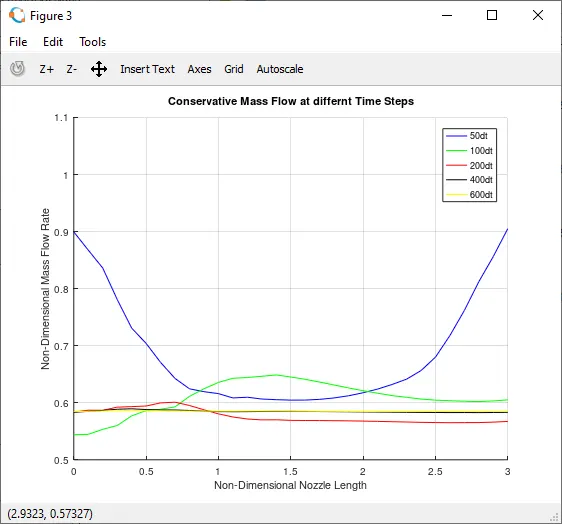
The mass flow at time step 50 to 100 is high. The mass flow reduced slowly and attained steady value at time step 400 to 600 range.

2. Mach number, Pressure, Density, Temperature distribution through Nozzle.

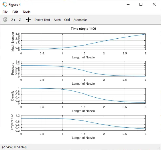
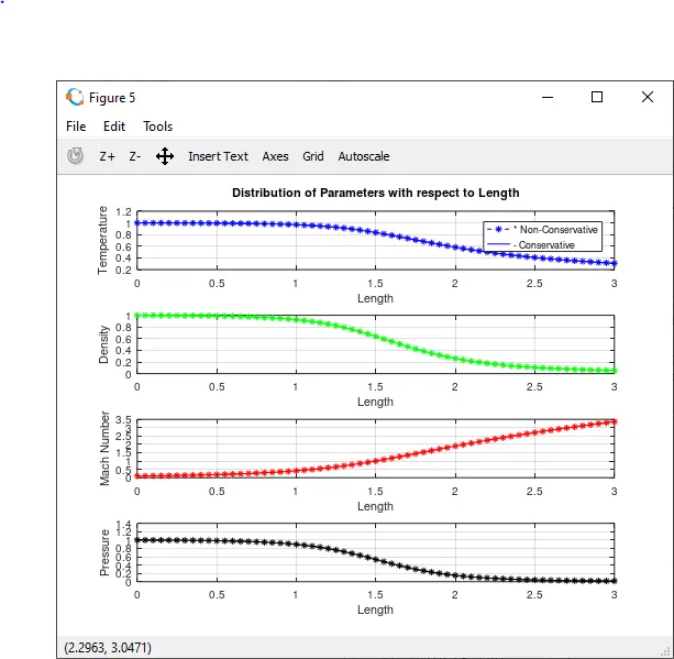
Non-Conservation vs Conservation Parameters

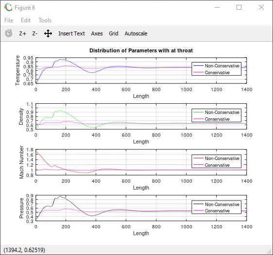
Non-Conservation vs Conservation Throat Parameters

The following plot shows the deviations of parameters at throat for both forms.

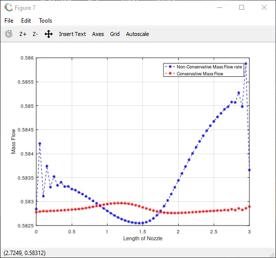
Non-Conservation vs Conservation Mass Flow

The following plot shows the mass flow rate of Non-Conservation and Conservation Forms.

Grid Independence

Comparison of Steady State results between Non-Conservative and Conservative.

	Density	Pressure	Temperature	Mach Number
Exact Solution	0.634	0.528	0.833	1.000
NonConservative (n=61 points)	0.63756	0.53261	0.83539	0.99970
Conservative (n=61points)	0.63826	0.53307	0.83519	0.99928
Non-Conservative (n=31 points)	0.63869	0.53424	0.83646	0.99937
Conservative (n=31points)	0.65069	0.54668	0.84017	0.98127

Conclusion:

1. Increase in grid points leads to more convergence time.

2. The variation of presure, temperature, velocity, density are same for both Conservative and Non-Conservative throughout the nozzle.

3. The change in grid points are resulted the same values for both forms, thus we can say the solution is grid independent.Thus, we can conclude that this is Grid Independent