Week 5 - Mid term project - Solving the steady and unsteady 2D heat conduction problem
AIM:
1.Solve the 2D heat conduction equation by using the point iterative techniques to the giben Boundary conditions for the problem by using:
i. Jacobi
ii. Gauss-seidel
iii. Successive over-relaxation
2. Write code for both implicit and explicit schemes (This is for the Transient Analysis only)
3. Write a detailed explanation for your results, plots or codes.
SOLUTION:
given,
Top Boundary = 600 K
Bottom Boundary = 900 K
Left Boundary = 400 K
Right Boundary = 800 K
absolute error = 1e-4
2DSteady State Heat Conduction Equation ==> d^2*T/dx^2 + d^2*T/dy^2 = 0
d^2*T/dx^2 = (T(i-1,j)-2T(i,j)+T(i+1,j))/Δx^2
d^2*T/dy^2 = (T(i,j-1)-2T(i,j)+T(i,j+1))/Δy^2
Tp = 1/k((TL+TR)/Δx^2) + 1/k((TT+TB)/Δy^2)
T(i,j) = 1/k((T(i-1,j)+T(i+1,j))/Δx^2) + 1/k((T(i,j-1)+T(i,j+1))/Δy^2)
where, k = 2*[(Δx^2+Δy^2)/(Δx^2)*(Δy^2)]
(1)Matlab Code to 2D Temperature distribution at Steady State:
%% Code to 2D Temperature distribution at Steady State
clear all
close all
clc

% Steady Flow Heat Conduction
% Inputs
nx = 50;
ny = 50;

% Relaxation factor
rf = 1.5;

% To calculate the values of x and y
x = linspace(0,1,nx);
dx = x(2)-x(1);
y = linspace(0,1,ny);
dy = y(2)-y(1);

% Assigning Boundary Conditions
T = ones(nx,ny);
T(1,:) = 600;     % Top Boundary
T(end,:) = 900;   % Bottom Boundary
T(:,1) = 400;     % Left Boundary
T(:,end) = 800;   % Right Boundary
k = 2*((dx^2+dy^2)/(dx^2*dy^2));

% Creating copy of T
Told = T;

%iterative_solver values from 1 to 3
iterative_solver = 1;

error = 9e9;
tol = 1e-4;

%jacobi method
tic
if iterative_solver == 1
    jacobi_iter = 1;
    while(error > tol)
        for i = 2:nx-1
            for j = 2:ny-1
                term1 = (Told(i+1,j)+Told(i-1,j))/(dx^2);
                term2 = (Told(i,j+1)+Told(i,j-1))/(dy^2);
                T(i,j) = (term1+term2)/k;
            end
        end
        error = max(max(abs(Told - T)));
        Told = T;
        jacobi_iter = jacobi_iter+1;
    end
    time1 = toc;
    figure(1)
    colormap(jet)
    contourf(x,y,T,'showText','on')
    xlabel('Xaxis')
    ylabel('Yaxis')
    title_text = sprintf('Iteration number = %d', jacobi_iter);
    title(title_text)
    colorbar
    pause(0.3)

end

%gs method
tic
if iterative_solver == 2
    gs_iter = 1;
    while(error > tol)
        for i = 2:nx-1
            for j = 2:ny-1
                term1 = (Told(i+1,j)+T(i-1,j))/(dx^2);
                term2 = (Told(i,j+1)+T(i,j-1))/(dy^2);
                T(i,j) = (term1+term2)/k;
            end
        end
        error = max(max(abs(Told - T)));
        Told = T;
        gs_iter = gs_iter+1;
    end
    time1 = toc;
    figure(2)
    colormap(jet)
    contourf(x,y,T,'showText','on')
    xlabel('Xaxis')
    ylabel('Yaxis')
    title_text = sprintf('Iteration number = %d', gs_iter);
    title(title_text)
    colorbar
    pause(0.3)

end


%SOR method
tic
if iterative_solver == 3
    sor_iter = 1;
    while(error > tol)
        for i = 2:nx-1
            for j = 2:ny-1
                term1 = (Told(i+1,j)+T(i-1,j))/(dx^2);
                term2 = (Told(i,j+1)+T(i,j-1))/(dy^2);
                T(i,j) = Told(i,j)*(1-rf) + rf*((term1+term2)/k);
            end
        end
        error = max(max(abs(Told - T)));
        Told = T;
        sor_iter = sor_iter+1;
    end
    time1 = toc;
    figure(3)
    colormap(jet)
    contourf(x,y,T,'showText','on')
    xlabel('Xaxis')
    ylabel('Yaxis')
    title_text = sprintf('Iteration number = %d', sor_iter);
    title(title_text)
    colorbar
    pause(0.3)

end
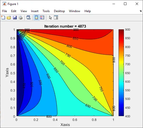
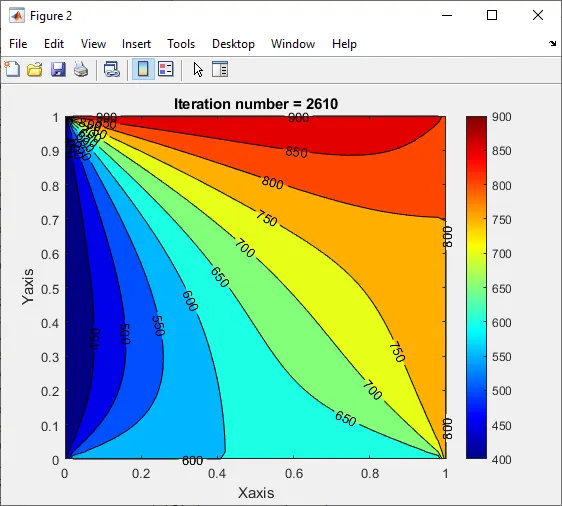
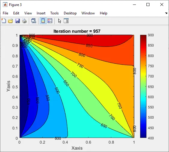
Results for Steady State as follows:
(1)Jacobi
(2)Gauss-Siedel
(3)SOR
(2)Unsteady State Heat Conduction:
2D UnSteady State Heat Conduction Equation ==> dT/dt = α*(d^2*T/dx^2 + d^2*T/dy^2)
d^2*T/dx^2 = (T(i-1,j)-2T(i,j)+T(i+1,j))/Δx^2
d^2*T/dy^2 = (T(i,j-1)-2T(i,j)+T(i,j+1))/Δy^2
Tp = 1/k((TL+TR)/Δx^2) + 1/k((TT+TB)/Δy^2)
T(i,j)^(n+1) = T(i,j)^n + k1*((T(i-1,j)-2T(i,j)+T(i+1,j))/Δx^2)+k2((T(i,j-1)-2T(i,j)+T(i,j+1))/Δy^2)
where,
k1 = α*(ΔT/Δx^2)
k2 = α*(ΔT/Δy^2)
Matlab Code for Explicit:
%% Code to 2D Temperature distribution at UnSteady State Explicit Mode
clear all
close all
clc

% Steady Flow Heat Conduction
% Inputs
nx = 50;
ny = 50;

% To calculate the values of x and y
x = linspace(0,1,nx);
dx = x(2)-x(1);
y = linspace(0,1,ny);
dy = y(2)-y(1);
dt = 0.01;

% alpha value
alpha = 1.5;

% Assigning Boundary Conditions
T = ones(nx,ny);
T(1,:) = 600;     % Top Boundary
T(end,:) = 900;   % Bottom Boundary
T(:,1) = 400;     % Left Boundary
T(:,end) = 800;   % Right Boundary

% K1 and k2
k1 = (alpha*dt)/(dx^2);
k2 = (alpha*dt)/(dy^2);
k = alpha*((dt/dx^2)+(dt/dy^2));

% Creating copy of T
Told = T;

%iterative_solver values from 1 to 3
iterative_solver = 1;

error = 9e9;
tol = 1e-4;

%Explicit method
tic
if iterative_solver == 1
    explicit_iter = 1;
    while(error > tol)
        for i = 2:nx-1
            for j = 2:ny-1
                term1 = (Told(i+1,j)+Told(i-1,j))*k1;
                term2 = (Told(i,j+1)+Told(i,j-1))*k2;
                T(i,j) = (Told(i,j)+(term1+term2))/(1+2*(k1+k2));
            end
        end
        error = max(max(abs(Told - T)));
        Told = T;
        explicit_iter = explicit_iter+1;
    end
    time = toc;
    figure(1)
    colormap(jet)
    contourf(x,y,T,'showText','on')
    xlabel('Xaxis')
    ylabel('Yaxis')
    title_text = sprintf('Iteration number = %d', explicit_iter);
    title(title_text)
    legend('Explicit Unsteady Heat Conduction', 'location', 'northoutside')
    colorbar
    pause(0.3)

end
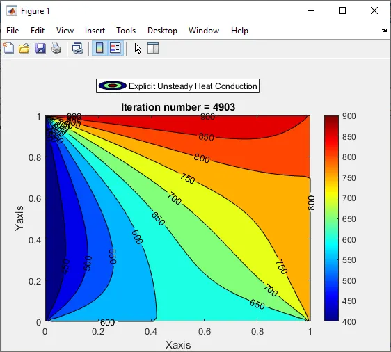
Results for Explicit:
Matlab Code for Unsteady Implicit:
%% Code to 2D Temperature distribution at UnSteady State Implicit Mode
clear all
close all
clc

% Steady Flow Heat Conduction
% Inputs
nx = 50;
ny = 50;

% To calculate the values of x and y
x = linspace(0,1,nx);
dx = x(2)-x(1);
y = linspace(0,1,ny);
dy = y(2)-y(1);
dt = 1/100;

% Relaxation factor
rf = 1.5;

% alpha value
alpha = 1.5;

% Assigning Boundary Conditions
T = ones(nx,ny);
T(1,:) = 600;     % Top Boundary
T(end,:) = 900;   % Bottom Boundary
T(:,1) = 400;     % Left Boundary
T(:,end) = 800;   % Right Boundary

% K1 and k2
k1 = (alpha*dt)/(dx^2);
k2 = (alpha*dt)/(dy^2);

% Creating copy of T
Told = T;
Tprev = T;
Tupd = T;

%iterative_solver values from 1 to 3
iterative_solver = 3;

error = 9e9;
tol = 1e-4;


%jacobi method
tic
if iterative_solver == 1
    jacobi_iter = 1;
    while(error > tol)
        for i = 2:nx-1
            for j = 2:ny-1
                term1 = (Told(i+1,j)+Told(i-1,j))*k1;
                term2 = (Told(i,j+1)+Told(i,j-1))*k2;
                T(i,j) = (Tprev(i,j)+(term1+term2))/(1+2*(k1+k2));
            end
        end
        error = max(max(abs(Told - T)));
        Told = T;
        jacobi_iter = jacobi_iter+1;
    end
    time1 = toc;
    figure(1)
    colormap(jet)
    contourf(x,y,T,'showText','on')
    xlabel('Xaxis')
    ylabel('Yaxis')
    title_text = sprintf('Iteration number = %d', jacobi_iter);
    title(title_text)
    legend('Jacobi Solver for 2D Unsteady Implicit Heat Conduction', 'location', 'northoutside')
    colorbar
    pause(0.3)

end

%gs method
tic
if iterative_solver == 2
    gs_iter = 1;
    while(error > tol)
        for i = 2:nx-1
            for j = 2:ny-1
                term1 = (Tupd(i+1,j)+Tupd(i-1,j))*k1;
                term2 = (Tupd(i,j+1)+Tupd(i,j-1))*k2;
                T(i,j) = (Tprev(i,j)+(term1+term2))/(1+2*(k1+k2));
                Tupd = T;
            end
        end
        error = max(max(abs(Told - T)));
        Told = T;
        gs_iter = gs_iter+1;
    end
    time1 = toc;
    figure(2)
    colormap(jet)
    contourf(x,y,T,'showText','on')
    xlabel('Xaxis')
    ylabel('Yaxis')
    title_text = sprintf('Iteration number = %d', gs_iter);
    title(title_text)
    legend('Gauss-Siedel Solver for 2D Unsteady Implicit Heat Conduction', 'location', 'northoutside')
    colorbar
    pause(0.3)

end


%SOR method
tic
if iterative_solver == 3
    sor_iter = 1;
    while(error > tol)
        for i = 2:nx-1
            for j = 2:ny-1
                term1 = (Tupd(i+1,j)+Tupd(i-1,j))*k1;
                term2 = (Tupd(i,j+1)+Tupd(i,j-1))*k2;
                T(i,j) = rf*(Tprev(i,j)+(term1+term2))/(1+2*(k1+k2))+(1-rf)*Told(i,j);
                Tupd = T;
            end
        end
        error = max(max(abs(Told - T)));
        Told = T;
        sor_iter = sor_iter+1;
    end
    time1 = toc;
    figure(3)
    colormap(jet)
    contourf(x,y,T,'showText','on')
    xlabel('Xaxis')
    ylabel('Yaxis')
    title_text = sprintf('Iteration number = %d', sor_iter);
    title(title_text)
    legend('SOR Solver for 2D Unsteady Implicit Heat Conduction', 'location', 'northoutside')
    colorbar
    pause(0.3)

end
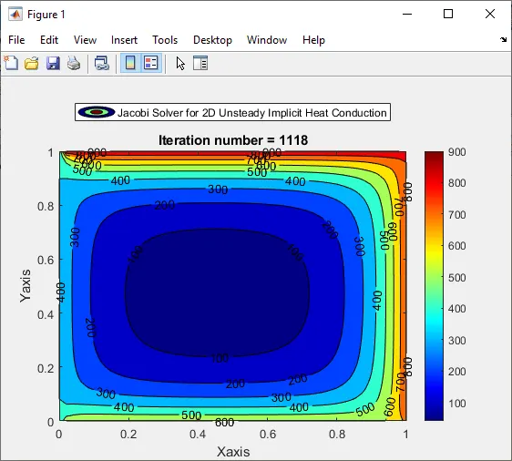
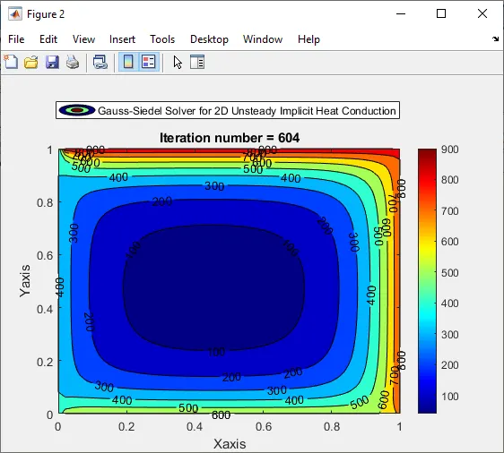
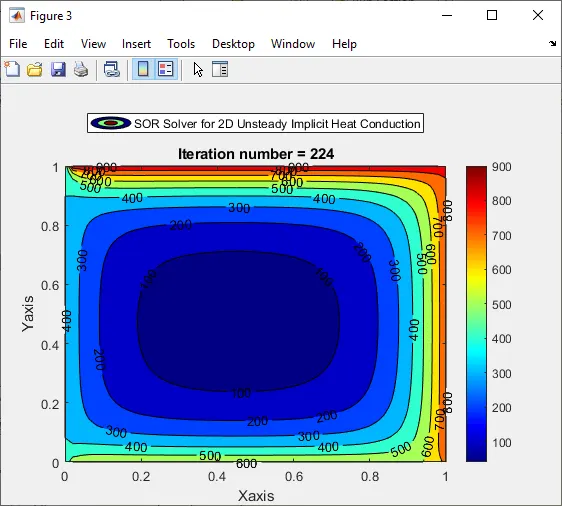
Results for Implicit:
1. Implicit Jacobi
2. Implicit Gauss-Siedel:
3. Implicit SOR:
Conclusion:
1. We see the iteration numbers for steady state for Jacobi, Gauss-Siedel and SOR. And for the simulation time, SOR is less and converges fast followed by Gauss-siedel and Jacobi.