Week 9 - FVM Literature Review

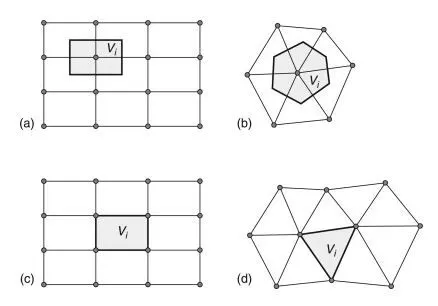
The finite volume method (FVM), like FEM, is based on an unstructured (e.g. triangular) mesh. Therefore, it is suitable for irregular and complex geometries. FVM has another advantage over FEM for fluid mechanic problems. By contrast, FVM is based on the integral form of the conservation laws, rather than their differential form. This leads to more accuracy/stability, especially for sharp gradients (i.e. large derivatives) inside a domain, which is also called the shock-capturing property. To explain this more clearly, as we mentioned before, the dynamics of flow can be described by the conservation of mass, momentum, and energy. These conservation laws can be written as a system of PDEs. Alternatively, conservation laws can be expressed by integral equations. For instance, the differential form of the continuity equation can be written as

`(delrho)/(delt) + (del(rhou))/(delx) + (del(rhov))/(dely) + (del(rhow))/(delz) = 0`

where u, v, and w are the components of flow velocities in the x, y, and z directions, and ρ is the density. The integral form of continuity for a control volume (or a finite volume) can be written as

`del/(delt) int_V rhodV + int_S rhou*dS = 0`

where V is the control volume, S is the control surface, u = (u, v, w), and S is the surface vector. Therefore, the change of mass inside a control/finite volume plus the net mass fluxes through the control surface should be zero. In FVM, the domain is first discretized into a number of nonoverlapping finite volumes or cells. Usually, these finite volumes are triangles (2D) or prisms (3D). Next, conservation laws are applied to each individual cell to form enough algebraic equations, which can be solved to compute the state variables.

Method of the CFD:

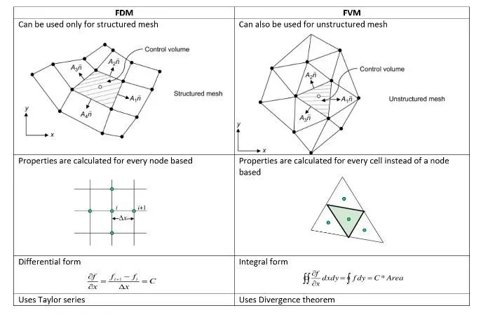
To solve the real-world problem, the people discovered three simples schemes for the numerical solution are

• Finite Difference Method
• Finite Element Method
• Finite volume Method

FEM has an important advantage in being able to deal with arbitrary geometries. The principal drawback, shared by any method that uses unstructured grids, is that the matrices of the linearized equations are not as well structured as those for regular grids making it more difficult to find efficient solution methods.

FEM is ideal for linear PDEs but expensive and complex for non-linear PDEs. Here higher-order accuracy is achieved by using a higher-order basis (i.e) shape functions. Extending to higher-order accuracy is relatively more complex than FVM and FDM. Higher-order accurate calculations are expensive in computation and Mathematical formulation, especially for non-linear PDEs. Mostly suitable for Heat transfer, Structural mechanics, vibrational analysis, etc. In FEM, the differential equation sometimes conservative law may be violated.

FVM can accommodate any type of grid, so it is suitable for complex geometries. The disadvantage of FVMs compared with FD schemes is that methods of order higher than a second are more difficult to develop in 3D. FVM is similar to FDM but the method (FVM) integrates the differential equation over a control volume and discretizes the domain. Since we have integrated the differential equation discretization is mathematically a valid one. It can be loosely viewed as FEM but the weight used in FVM is 1. In FVM, fluxes are integrated and the resultant is set to zero, so flux is conserved. FVM handles almost any PDEs and complex domains. Interpolation done from face to center will reduce the accuracy of this process. FVM accuracy is based on the order of the polynomial used. FVM can also produce any order-accurate numerical solution similar to FDM. The main difference between the FVM and other numerical methods is its high flexibility in implementing the discretization method. In the FVM, the discretization process is carried out directly in the physical domain without any transformation between the computational and physical coordinate systems. In addition, FVM is a strictly conservative method.

Finite Difference Method: It is difficult to satisfy conservation and to apply for irregular geometries

Finite Volume Method: It tends to be biased toward edges and one-dimensional physics.

Finite Element Method: It is difficult to solve hyperbolic equations using FEM.

A commercial package such as FLUENT uses Finite Volume Method.

Interpolation Schemes in Finite Volume Method (FVM):

The interpolation schemes used in the FVM method are as follows:

1. Upwind Interpolation Scheme. (UDS)
2. Central Differencing Approximation. (CDS)
3. Quadratic Upwind Differencing Scheme. (QUICK)
4. Hybrid Interpolation Scheme. (CDS & UDS)
5. Total variation Diminishing Scheme. (TVD)

we need the evaluation of surface and volume integrals in our finite volume formulation. Still, the surface, as well as volume integrals, require the value of the unknown variable at locations other than the computational notes of the CV. So somehow we have to cover with some sort of schemes or mathematical approximation to compute the values at these locations, and that is why we need various types of interpolation formulae. Now the various possibilities for interpolation include upwind interpolation, linear interpolation, quadratic upwind interpolation, recently developed hybrid schemes, TVD that is Total Variation Dimensions schemes, and ENO Essentially Non-Oscillatory interpolation schemes.

Upwind Interpolation Scheme(UDS):

The upwind interpolation (UDS) for approximating the value of a variable f at the east face of a control volume is given

`f_e = {(f_p,if,(v.n)_e,>,0),(f_E,if,(v.n)_e,<,0):}`

Here, we would require an upwind interpolation scheme it is essentially used for what we called convection dominated problems, and here the velocity at a given point direction of that velocity that determines the variable values to be used in the interpolation process, the name upwind refers to that we are going to make use of the node which is upwind or upstream of the given node.

UDS is equivalent to using a backward or forward finite difference approximation(depending on the flow direction). It is the first-order accurate scheme and is numerically diffusive with a coefficient of numerical diffusion

`Gamma_e^(n)=((rhou)_eDeltax)/2`

The scheme is developed from the convective flows with the suppressed diffusion effects.

The advantages of this scheme? Now upwind interpolation is the only approximation that satisfies the boundedness criterion unconditionally, unconditionally in the sense that respect irrespective of what the velocity values are and irrespective of what the grid spacing the solution will always remain bounded that is this use of upwind interpolation will never yield oscillatory solutions.

This advantage is coupled with disadvantages. The first one is numerical diffusive, if we have got sharp peaks or oscillatory values which are actually present in the solution those would be damped out because of the presence of numerical diffusion, so the numerical diffusion is magnified in multi-dimensional flows, especially of the flow is oblique to the grid space. And peaks or rapid variations in the variables will be smeared out because of the introduction of an additional diffusive coefficient what we called a numerical diffusive coefficient by the use of upwind interpolation schemes, and we have already seen that it is only the first-order accurate.
Hence, we require very fine grids to obtain an accurate solution, but nevertheless the advantage this scheme provides is the use the unconditional stability specifically for advection-dominated problems.

UDS scheme is very popular we can go for a very fine grid and we can rest assured that we will
not get a solution that becomes unbounded.

Linear Interpolation Scheme:

The interpolation scheme commonly used is Linear interpolation and in short, it is called CDS which is Central Difference Scheme, we will see very shortly what is the correlation between the central difference scheme which we have learned earlier in the finite difference module, and the simple linear interpolation. So now here we have approximated the value of a variable at the control volume face center by linear interpolation of the values at the two nearest computational nodes.

So for instance, if you are looking at the east face so function value at the east face would be a linear interpolation for the function value at the capital E which is the eastern node, and the current node P, and we use a waiting function a lambda e this lambda e would depend on the relative locations of the computational nodes capital E and capital P with respect to the eastern face. So fe=f at E*lambda e+fP 1-lambda e where lambda is given by xe-x capital P/x capital E-xP. Now, this linear interpolation is equivalent to the use of the central difference formula of the first-order derivative. Hence, this scheme is also termed a central difference scheme or CDS.

The value of the variable at the CV face center is approximate from the values near two computational nodes. In this location at 'e' on a cartesian grid, the variable value is approximated by,

`f_e=f_E(lambda_e)+f_p(1-lambda_e)`

`lambda_e = (x_e-x_p)/(x_E-x_p)`

The characteristic of scheme CDS is second-order accuracy, so from now onwards you refer to linear interpolation by its short acronym that is CDS, it is second order accurate the accuracy is very good but we might have one small problem for advection-dominated situations, and this scheme may produce oscillatory solutions, so that is the negative side. On the positive node, it is the simplest and the most widely used interpolation.

We need to worry about the oscillatory only if the grid spacing is very large, with a small grid spacing we do not have to worry about the oscillation present and in that case, CDS gives us a choice of a very good and very simple second-order accurate scheme, so that is the reason why? It is used very commonly, especially in flow simulation which requires the use of the finite spatial and temporal grid for instance, if you are looking at the simulations of turbulent flows using largely simulation or direct numerical simulation approach.

Quadratic Upwind interpolation(QUICK):

Our next, scheme is what we called the quadratic upwind interpolation scheme, we had a look at the upwind scheme which was first-order accurate, we said it takes care of the presence of the high velocity or the advective fluxes, we do not have to worry about introducing oscillatory solutions, but the downside is UDS is only first-order accurate. Then we had a look at linear integration, linear interpolation is second-order accurate but it is prone to producing oscillation solutions. So the next thing was we can get a second-order accurate scheme, which has got better damping properties than CDS and it is got better accuracy than UDS, so this quick upwind interpolation scheme was devised for this particular purpose, the name upwind which is still here that tells us we are going to get more prominence or more weightage to the function values at the nodes which are on the upstream side okay.

So now let us have a look at the eastern face, so approximate the value of the variable at the CV face center by using quadratic interpolation of the values at the 3 nearest computational nodes, and which will be these 3 nearest computational nodes? We are going to use one downstream node let us denote by capital D and 2 upstream nodes by capital U and capital UU, in this generalized description we are going to use capital P or E or capital W. Which we normally used to denote our computational nodes on the eastern and western sides, because it depends on the direction of the flow velocity, for instance, if you are looking at a flow in positive x direction at this cell face e, then our upstream node will become the capital P and downstream nodes will become capital U is identical with capital E and UU becomes capital EE that is east to west. So now first let us have a look at this generic formula fe=f capital U+g1 times fD-fU + g2 times fUU-fU, where these coefficients g1 and g2 are based on the mesh spacings xe-xU xexUU/xD-xU times x capital D-xUU. And g2 similarly, given as xe-x capital U times xe-xD/xUU-xU times x UU-xD.

This scheme is QUICK, the QUICK is basically an acronym that stands for Quadratic of Upwind Interpolation for Convective Kinematics, convective kinematics because this particular interpolation would be
used for the convection-dominated problem, and quadratic because we have obtained this interpolation based on what quadratic interpolation formula. And upwind because is there because we used 3 nodes 1 downstream and 2 upwind that is why? This is named quadratic upwind interpolation for convective kinematics. Now, this particular scheme is third-order accurate in both uniform and non-uniform grids, and in case we had a uniform grid we get a very simplified form that phi at e=6/8 phi at upstream node+ 3/8 phi at downstream node-1/8 phi the function value at upstream to the upstream node. Now because of the third-order accuracy, this scheme is again very popular in modeling advection-dominated problems, but note here that still there are some issues with oscillations that are parallel and similar not as severe as the central difference scheme, but nevertheless there are some possibilities of obtaining unwanted oscillations in the numerical solutions with the use of quadratic upwind interpolation scheme. It is also represented as the QUICK Interpolation. The quick interpolation on a uniform cartesian grid is given by

`phi_e=6/8phi_U+3/8phi_D-1/8phi_(UU)`

Advantages:

• It is the better version of UDS and CDS because it is more accurate than UDS and more damping in nature than CDS as it uses 3 nodes to solve.
• It is of 3rd order accurate.

Disadvantages:

• The use of QUICK can lead to subtle problems caused by such unbounded results.
• Implementation of boundary conditions can be problematic with such higher-order schemes.

Flux Limiters:

Flux limiters are used in the numerical schemes to solve problems of fluid dynamics, described by highly coupled non-linear Partial Differential Equations. If we tend to use low-order numerical schemes for the solving of the governing equations then we might get a highly oscillatory and unstable solution near the discontinuity if present. Whereas if we tend to use higher-order numerical schemes to capture the phenomenon more accurately we tend to exploit the computational power unnecessarily. The main idea behind the use of flux limiters is to limit the spatial derivative terms near the discontinuities to physical real values so as to maintain physical consistency. There are several types of flux/slope limiter functions. They come in handy when sharp wave-fronts/peaks are present. For smoothly changing waves/functions, the flux limiters do not operate and the spatial derivatives can be represented normally.

It is imperative to note that flux limiters are also referred to as slope limiters because they both have the same mathematical form, and both have the effect of limiting the solution gradient near shocks or discontinuities.

`F(u_(i+1/2)) = f^(low)(i+1/2) - ϕ(r_i)(f^(low)(i+1/2)-f^(high)(i+1/2))`

`F(u_(i-1/2)) = f^(low)(i-1/2)- ϕ(r_i-1)(f^(low)(i-1/2)-f^(high)(i-1/2))`

here

`f^(low)` = Low precision flux (1st order precise)`

`f^(high)`= High precision flux (Highest order precision)`

`ϕ(r) = Flux limiter function and r = (u_i-u_(i-1))/(u_(i+1)-u_i)`

Conclusion:

The finite Volume Method (FVM) is really a powerful approach to solving CFD problems. With the help of proper interpolation schemes and the accurate use of flux limiters in case of any discontinuities present, we can solve a wide range of CFD problems.

Though it may be difficult to code and implement it on the computer it gives the added advantage of its robustness.