Week 3 - Solving second order ODEs
Aim:
Program to solve second-order differential equations using Matlab.
By taking an example of a simple pendulum in the program.
The way the pendulum moves depends on Newton's second law. When this law is written down, we get a second-order Ordinary Differential Equation that describes the position of the "ball" w.r.t time.
Similarly, hundreds of ODEs describe vital phenomena, and if we can solve these equations, we will be able to simulate any of these systems.
Govering equation:
`(d^2theta)/dt^2` + `b/m` `(d theta)/dt` + `g/l` `sin theta` = `0`
Our objective is to write a program that solves the following ODE. This ODE represents the equation of motion of a simple pendulum with damping. In the above equation,
g = gravity in m/`s^2`,
L = length of the pendulum in m,
m = mass of the ball in kg,
b = damping coefficient.
To solve the above equation of ODE we have to reduce the order of the equation to lower order.
Let,
`theta = theta_1`
`(d theta)/dt = (d theta_1)/dt` = `theta_2` ----------- (1)
`(d^2 theta)/dt^2 = (d^2theta_1)/dt^2 = d/dt((d theta_1)/dt) = d/dt(theta_2)` ------------- (2)
`(d^2theta)/dt^2` + `b/m` `(d theta)/dt` + `g/l` `sin theta` = `0`
`(d^2theta_1)/dt^2` + `b/m` `(d theta_1)/dt` + `g/l` `sin theta_1` = `0`
`(d theta_2)/dt + b/m theta_2 + g/l sintheta_1 = 0` ------------------------------- (3)
`(d theta_2)/dt = -( b/m theta_2 + g/l sintheta_1)` -------------------------------- (4)
The simple differential equations are written in the form of a matrix called solution vector.
`d/dt [[theta_1],[theta_2]] = [[theta_2],[( -b/m theta_2 )-(g/l sintheta_1)]]` ---------------- (5)
`d/dt [[theta_1],[theta_2]] = theta` ---------------------- (6)
With the help of the above equation, we can solve the problems of a simple pendulum in Matlab by writing code.
Inputs for first program, where we are going to plot a graph between displacement and velocity with the help of function.
length of pendulum string (l) = 1 meter
mass of bob (m) = 0.1 kg
damping coefficient (b) = 0.05
gravity = 9.81 m/`s^2`
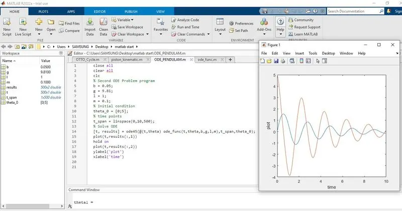
% Program to solve Second ODE problems
% Input

b = 0.01; % damping coefficient
g = 9.81; % gavity in m/s^2
l = 1;    % Length of pendulum string in meter
m = 0.1;  % Mass of in kg

% Initial condition
theta_0 = [0;5];

% time points
t_span = linspace(0,10,500);

% ODE 45 function to solve second order ode
[t, results] = ode45(@(t,theta) ode_func(t,theta,b,g,l,m),t_span,theta_0);

% Plotting of results
plot(t,results(:,1))
hold on
plot(t,results(:,2))
ylabel('plot')
xlabel('time')
% ODE 45 function to solve second order ODE

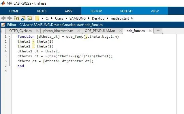
function [dtheta_dt] = ode_func(t,theta,b,g,l,m)
theta1 = theta(1)
theta2 = theta(2)
dtheta1_dt = theta2;
dtheta2_dt = -(b/m)*theta2-(g/l)*sin(theta1);
dtheta_dt = [dtheta1_dt;dtheta2_dt];
end
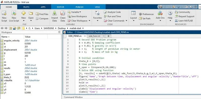
% Second ODE Problem program
b = 0.05; % Damping coefficient
g = 9.81; % gravity in m/s^2
l = 1;    % length of pendulum string in meter
m = 1;    % mass of bob in kg

% Initial condition
theta_0 = [0;3];
% time points
t_span = linspace(0,20,200);
% Solve ODE using function
[t, results] = ode45(@(t,theta) ode_func(t,theta,b,g,l,m),t_span,theta_0);
figure('Name','Graph between time, displacement and angular velocity','NumberTitle','off')
plot(t,results(:,1))
hold on
plot(t,results(:,2))
ylabel('Displacement and Angular velocity')
xlabel('Time')
legend('displacement','angular velocity')
grid on
hold off
% To create animation of simple pendulam
displacement = results(:,1);
angular_velocity = results(:,2);
ct=1;
for i = 1:length(displacement)
    % initial coordinates
    x0 = 0;
    y0 = 0;

    % last coordinates
    x1 = 1-1*sin(displacement(i));
    y1 = 1-1*cos(displacement(i));

    % Creating annimation
    figure('Name','Animation of simple pendulum','NumberTitle','off')
    % Base of pendulum
    plot([0 2],[1 1],'linewidth',4,'Color','g')
    hold on
    % bob of pendulum and String of pendulam
    plot([1 x1],[1 y1],[x1 x1],[y1 y1],'o','MarkerSize',15,'MarkerFaceColor','k','linewidth',3)
    hold on
    plot(x0,y0,'MarkerSize',3,'MarkerFaceColor','b')

    % axis setting
    axis([0 2 -0.5 2])
    pause(0.03)
    M(ct)=getframe(gcf);
    hold off
    ct=ct+1;

end

% Movie from captured frames
movie(M)
videofile = VideoWriter('Second_ode45_Simple_Pendulum.AVI','Uncompressed AVI');
open(videofile)
writeVideo(videofile,M)
close(videofile)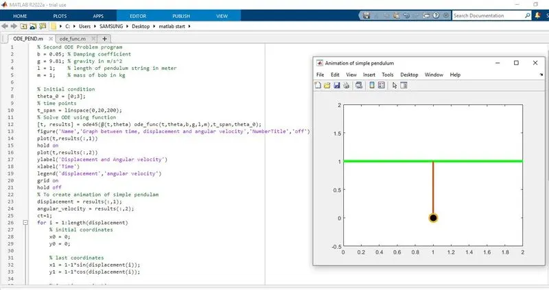
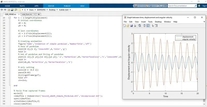
Output:
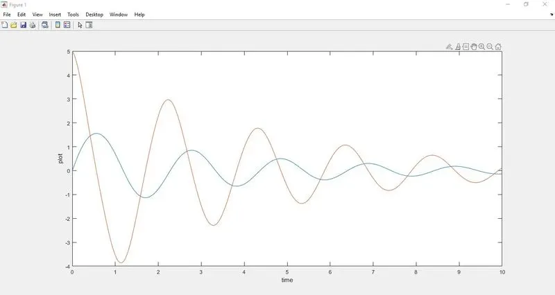
A graph is Plotted between the time, angular velocity, and displacement of the motion of the simple pendulum.
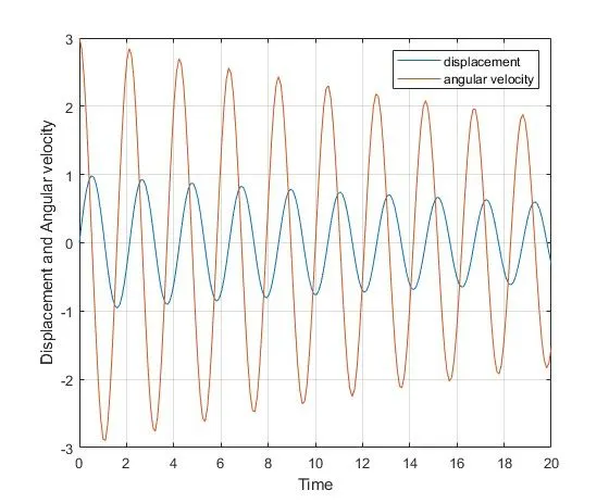
The blue color curve is representing the displacement of the bob, which is starting from 0. The red color curve is representing the angular velocity of the bob, which starts from 3 rad/sec. At the end of the t_span, both the angular velocity and displacement become zero.
Results:
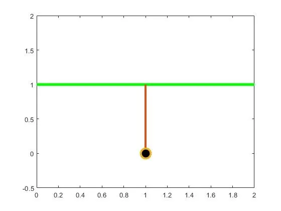
Animation of a simple pendulum using the ode45 solver has been generated and the link is attached below. Animation is made up of capturing the different positions of the bob and by connecting all the points of bob, the motion of a simple pendulum is created. here we reduced the second order differential equation to a simple differential equation.
YOUTUBE LINK:- https://youtu.be/8fH8kBU3wxA