Project 2 - Rankine cycle Simulator

Aim

The program's main objective is to obtain all the values at all different state points and plot the T-S & H-S curves for the Rankine cycle and calculate the state functions at different states, utilizing the steam table.

Rankine Cycle

The Rankine cycle or Rankine Vapor Cycle is the process widely used by power plants such as coal-fired power plants or nuclear reactors. In this mechanism, a fuel is used to produce heat within a boiler, converting water into steam which then expands through a turbine producing helpful work. This process was developed in 1859 by Scottish engineer William J.M. Rankine. This is a thermodynamic cycle that converts heat into mechanical energy—which usually gets transformed into electricity by electrical generation.

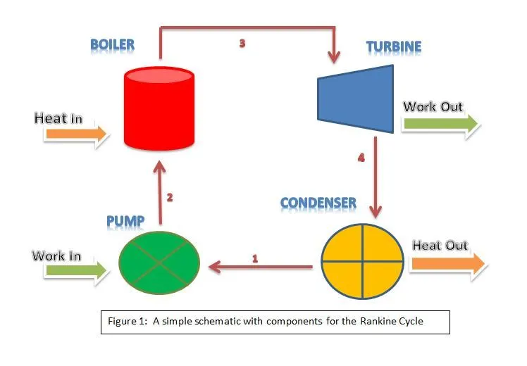
The steps in the Rankine Cycle as shown in (Figure 1) and the corresponding steps in the pressure-volume diagram (Figure 2) are outlined below:

Pump: Compression of the fluid to high pressure using a pump (this takes work)

Boiler: The compressed fluid is heated to the final temperature (at boiling point), therefore, a phase change occurs—from liquid to vapor.

Turbine: Expansion of the vapor in the turbine.

Condenser: Condensation of the vapor in the condenser (where the waste heat goes to the final heat sink (the atmosphere or a large body of water (Ex. Lake or river).

Process 3-4: Isentropic Expansion:

The vapor is expanded in the turbine, thus producing work that may be converted to electricity. In practice, the expansion is limited by the temperature of the cooling medium and by the erosion of the turbine blades by liquid entrainment in the vapor stream as the process moves further into the two-phase region. Exit vapor qualities should be greater than 90% to avoid blade erosion.

Process 4-1: Isobaric Heat Rejection:

The vapor-liquid mixture leaving the turbine is condensed at low pressure, usually in a surface condenser using cooling water. In well-designed and maintained condensers, the pressure of the vapor is well below atmospheric pressure, approaching the saturation pressure of the operating fluid at the cooling water temperature.

Process 1-2: Isentropic Compression:

The pressure of the condensate is raised in the feed pump. Because of the low specific volume of liquids, the pump work is relatively small and often neglected in thermodynamic calculations.

Process 2-3: Isobaric Heat Transfer:

High-pressure liquid enters the boiler from the feed pump and is heated to the saturation temperature. Further addition of energy causes evaporation of the liquid until it is fully converted to saturated steam.

Work done on the pump, per kg of water: WP= `h_2` – `h_1`

Energy added in steam generator: `q_1` = `h_3` – `h_2`

Work delivered by turbine: WT= `h_3` – `h_4`

Energy rejected in the condenser, `q_2` = `h_4 - h_1`

The thermal efficiency of the Rankine cycle is given by:

h1,h2,h3,h4 are the enthalpy at the respective state points.

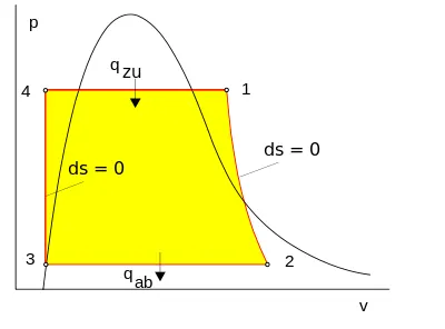
The pressure-volume diagram of the Rankine cycle. This illustrates the changes in pressure and volume the working fluid (water) undergoes to produce work.

The efficiency of the Rankine cycle is limited by the high heat of vaporization by the fluid. The fluid must be cycled through and reused constantly; therefore, water is the most practical fluid for this cycle. This is not why many power plants are located near a body of water—that's for the waste heat.

As the water condenses in the condenser, waste heat is given off in the form of water vapor—which can be seen billowing from a plant's cooling towers. This waste heat is necessary for any thermodynamic cycle. Due to this condensation step, the pressure at the turbine outlet is lowered. This means the pump requires less work to compress the water—resulting in higher overall efficiencies.

Reheating of Steam

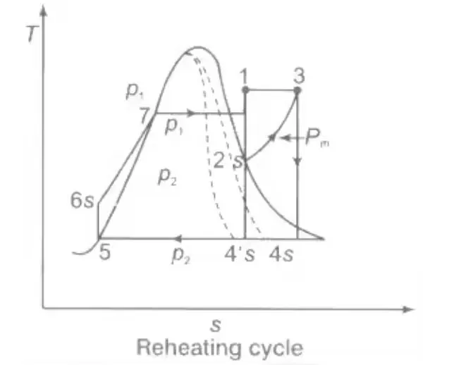
In such cases all the steam after partial expansion in the turbine is brought back to the boiler, reheated by combustion gases, and fed back to the turbine for further expansion. This is known as Reheating.

The main objective of the reheat cycle is to limit the quality of steam at the turbine outlet.

Cycle efficiency improves with reheat; however, the cycle efficiency in a single reheat plant is influenced by the pressure at which steam is reheated.

The efficiency increases as the reheat pressure are lowered and reaches a peak at a pressure ratio between 0.20 and 0.25.

Reheating steam also increases the net work output of the turbine.

Advantages of Re‑heating

Due to reheating, the net-work done increases.

Heat supply increases.

The thermal efficiency may increase or decrease depending upon the mean temperature of heat addition.

Due to reheating, the turbine exit dryness fraction increases so moisture decreases ‑ so blade erosion becomes minimum ‑ so the life of the turbine will be increased.

Regeneration

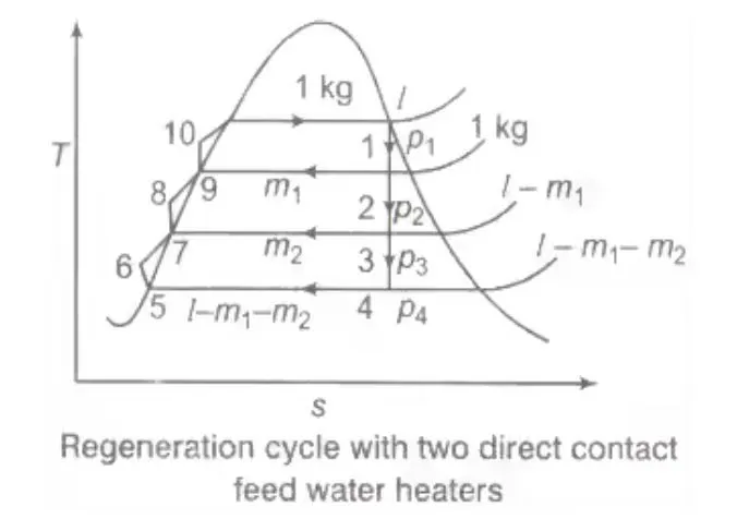
The mean temperature of heat addition (and so efficiency) can also be increased by reducing the amount of heat added at low temperatures in the economizer section of the steam generator.

In the regeneration process energy is exchanged internally between the expanding fluid in the turbine and the compressed fluid before heat addition.

An ideal regenerative cycle does not affect work output from the turbine, it is more efficient with a high steam rate.

Reheating of steam improved the thermal efficiency of the plant, the net work output of the turbine, and reduction in blade erosion (or quality of steam improve).

By regeneration thermal efficiency of the plant can be increased but it does not affect work output from the turbine.

The efficiency of Steam Power Plant: Overall efficiency of the steam per plant is given by

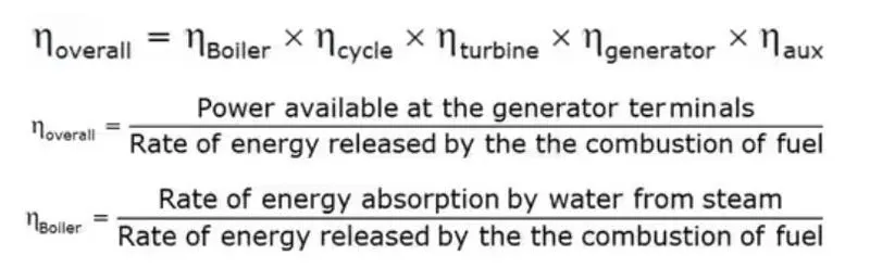
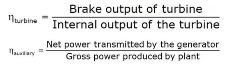
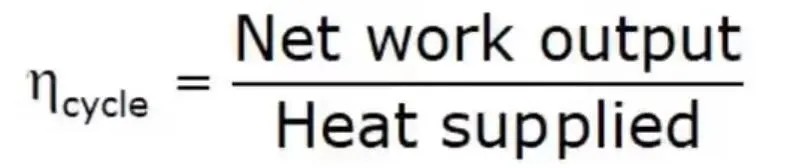
Specific steam consumption (SSC): It is the amount of steam required to produce unit work.

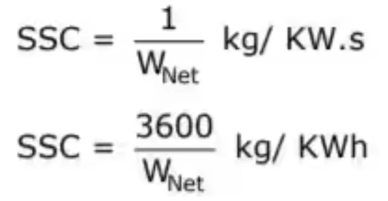
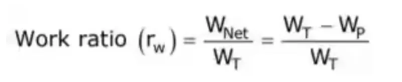
Work ratio (rw): It is the ratio of the net-work to turbine work.

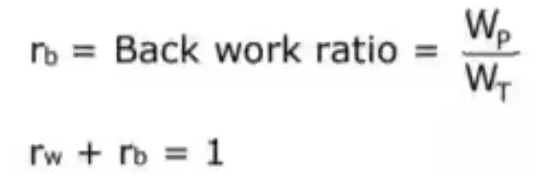
Back work ratio (rbw): It is the ratio of the pump work to the turbine work.

Combined Cycle Power Generation

It is an assembly of heat engines that works with the same source of heat. The principle of combined cycle power generation is that the exhaust of one heat engine is used as the source of heat for another heat engine. This process increases the overall efficiency of a heat engine.

Advantages of Regeneration Cycle

Heat supplied to boiler becomes reduced

Thermal efficiency increases since the average temperature of heat added to the cycle increases.

Due to bleeding in the turbine, erosion of the turbine due to moisture is reduced.

Objective:

By entering the given data, calculate the state points of the Rankine cycle at different state points including enthalpy and entropy of the system. with the help of the XSteam table and the thermodynamic equations the various states variables such as Pressure, Temperature, Enthalpy, and Entropy are calculated.

Then calculate the performance parameters of the given Rankine cycle.

Draw a T-S and H-S graph diagram from the data.

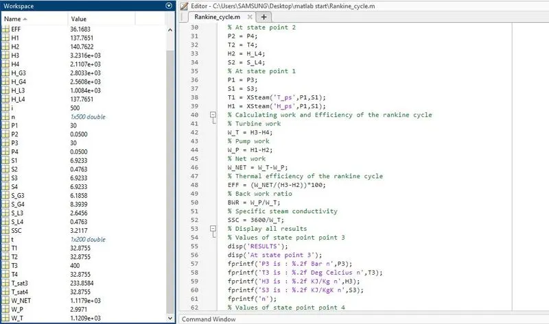
% Program Rankine cycle
disp('RANKINE CYCLE SIMULATOR');
disp('1-2 is Isentropic Compression in the Pump');
disp('2-3 Isobaric Heat Transfer in the Boiler');
disp('3-4 is Isentropic Expansion in the Turbine');
disp('4-1 Isobaric Heat Rejection in the Condenser');

% Given Inputs
P3 = input('Enter the pressure at the Turbine Inlet(in bar): ');
T3 = input('Enter the Temperature at the Turbine Inlet(in Degree Celcius): ');
P4 = input('Enter the pressure at the Condenser Inlet(in bar): ');

% Calculating the value of P,T,H,S at each state points
% At state point 3
H3 = XSteam('h_pT',P3,T3);
S3 = XSteam('h_pT',P3,T3);
H_L3 = XSteam('hL_p',P3);
H_G3 = XSteam('hV_p',P3);
S_L3 = XSteam('sL_p',P3);
S_G3 = XSteam('sV_p',P3);
T_sat3 = XSteam('Tsat_p',P3);

% At state point 4
S4 = S3;
S_L4 = XSteam('sL_p',P4);
S_G4 = XSteam('sV_p',P4);
D = (S4-S_L4)/(S_G4-S_L4); % Calculating the dryness fraction
H_L4 = XSteam('hL_p',P4); % Calculating the enthalpy at point 4
H_G4 = XSteam('hV_p',P4);
T4 = XSteam('T_ph',P4,H4);
T_sat4 = XSteam('Tsat_p',P4);

% At state point 2
P2 = P4;
T2 = T4;
S2 = S_L4;
H2 = XSteam('H_ps',P2,S2);

% At state point 1
P1 = P3;
S1 = S3;
H1 = H_L4;
T1 = XSteam('T_ps',P1,S1);

% Calculating work and Efficiency of the rankine cycle
% Turbine work
W_T = H3-H4;

% Pump work
W_P = H2-H1;

% Net work
W_NET = W_T-W_P;

% Thermal efficiency of the rankine cycle
EFF = (W_NET/(H3-H2))*100;

% Back work ratio
BWR = W_P/W_T;

% Specific steam conductivity
SSC = 3600/W_T;

% Display all results
% Values of state point point 3
disp('RESULTS');
disp('At state point 3');
fprintf('P3 is : %.2f Bar n',P3);
fprintf('T3 is : %.2f Deg Celcius n',T3);
fprintf('H3 is : %.2f KJ/Kg n',H3);
fprintf('S3 is : %.2f KJ/KgK n',S3);
fprintf('n');

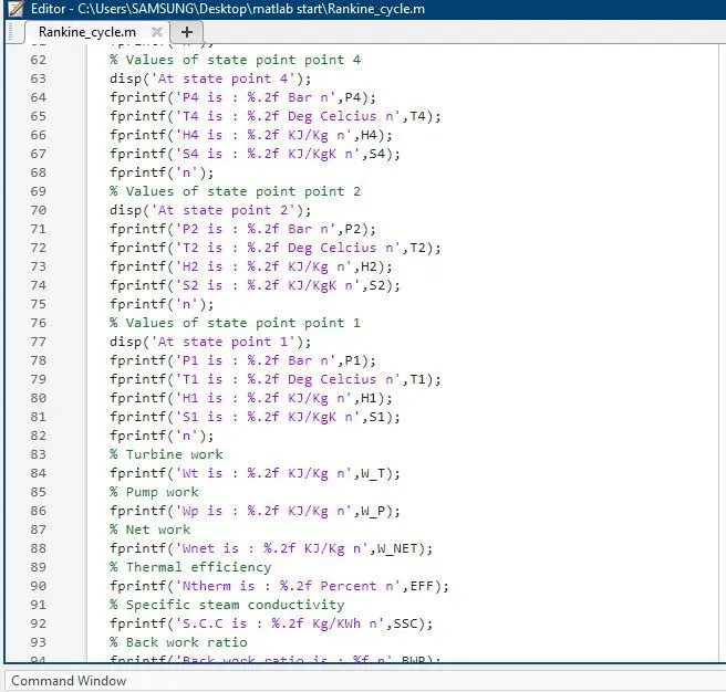
% Values of state point point 4
disp('At state point 4');
fprintf('P4 is : %.2f Bar n',P4);
fprintf('T4 is : %.2f Deg Celcius n',T4);
fprintf('H4 is : %.2f KJ/Kg n',H4);
fprintf('S4 is : %.2f KJ/KgK n',S4);
fprintf('n');

% Values of state point point 2
disp('At state point 2');
fprintf('P2 is : %.2f Bar n',P2);
fprintf('T2 is : %.2f Deg Celcius n',T2);
fprintf('H2 is : %.2f KJ/Kg n',H2);
fprintf('S2 is : %.2f KJ/KgK n',S2);
fprintf('n');

% Values of state point point 1
disp('At state point 1');
fprintf('P1 is : %.2f Bar n',P1);
fprintf('T1 is : %.2f Deg Celcius n',T1);
fprintf('H1 is : %.2f KJ/Kg n',H1);
fprintf('S1 is : %.2f KJ/KgK n',S1);
fprintf('n');

% Turbine work
fprintf('Wt is : %.2f KJ/Kg n',W_T);

% Pump work
fprintf('Wp is : %.2f KJ/Kg n',W_P);

% Net work
fprintf('Wnet is : %.2f KJ/Kg n',W_NET);

% Thermal efficiency
fprintf('Ntherm is : %.2f Percent n',EFF);

% Specific steam conductivity
fprintf('S.C.C is : %.2f Kg/KWh n',SSC);

% Back work ratio
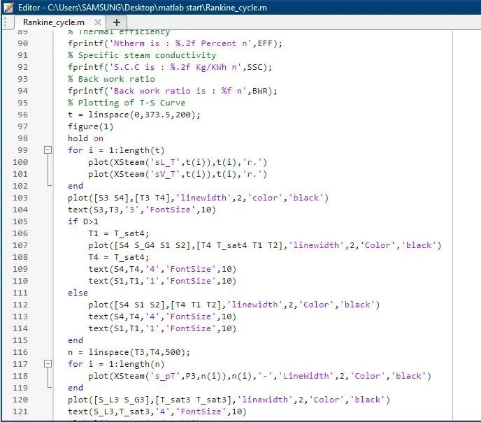
fprintf('Back work ratio is : %f n',BWR);

% Plotting of T-S Curve
t = linspace(0,373.5,200);
figure(1)
hold on
for i = 1:length(t)
    plot(XSteam('sL_T',t(i)),t(i),'r.')
    plot(XSteam('sV_T',t(i)),t(i),'r.')
end
plot([S3 S4],[T3 T4],'linewidth',2,'color','black')
text(S3,T3,'3','FontSize',10)
if D>1
    T1 = T_sat4;
    plot([S4 S_G4 S1 S2],[T4 T_sat4 T1 T2],'linewidth',2,'Color','black')
    T4 = T_sat4;
    text(S4,T4,'4','FontSize',10)
    text(S1,T1,'1','FontSize',10)
else
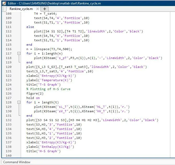
    plot([S4 S1 S2],[T4 T1 T2],'linewidth',2,'Color','black')
    text(S4,T4,'4','FontSize',10)
    text(S1,T1,'1','FontSize',10)
end
n = linspace(T3,T4,500);
for i = 1:length(n)
    plot(XSteam('s_pT',P3,n(i)),n(i),'-','LineWidth',2,'Color','black')
end

plot([S_L3 S_G3],[T_sat3 T_sat3],'linewidth',2,'Color','black')
text(S_L3,T_sat3,'4','FontSize',10)
xlabel('Entropy(KJ/Kg-k)')
ylabel('Temperature(K)')
title('T-S Graph')

% Plotting of H-S Curve
figure(2)
hold on
for i = length(t)
    plot(XSteam('sL_T',t(i)),XSteam('hL_T',t(i)),'r.')
    plot(XSteam('sV_T',t(i)),XSteam('hV_T',t(i)),'r.')
end

plot([S3 S4 S1 S2 S3],[H3 H4 H1 H2 H3],'LineWidth',2,'Color','black')
text(S3,H3,'3','FontSize',10)
text(S4,H3,'4','FontSize',10)
text(S1,H3,'1','FontSize',10)
text(S2,H3,'2','FontSize',10)
xlabel('Entropy(KJ/Kg-K)')
ylabel('Enthalpy(KJ/Kg)')
title('H-S Graph')

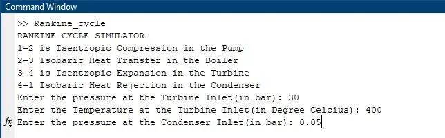
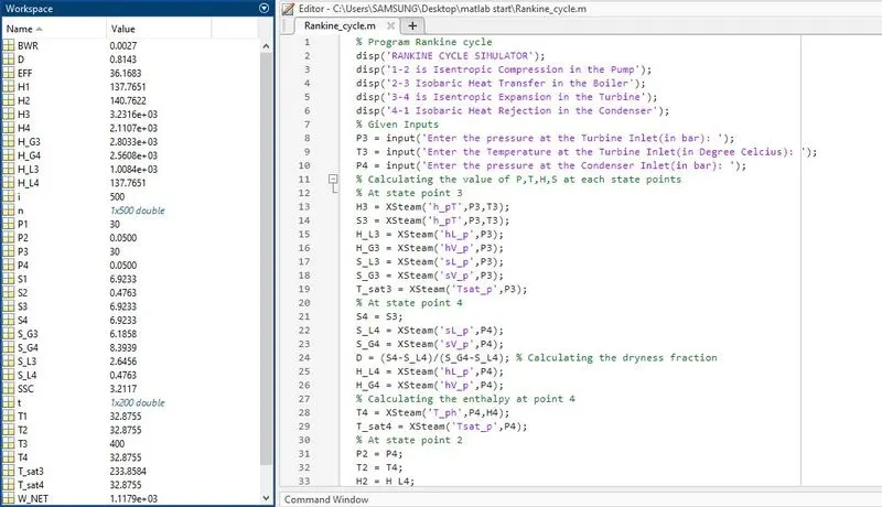
Output: The Rankine cycle plots have been generated by calculating the state points, Network output and efficiency, and the output is printed in the command window.

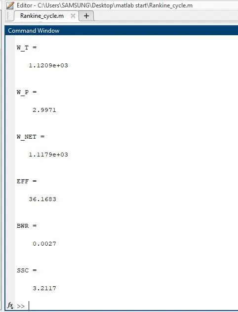
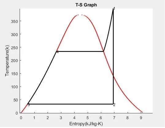
The performance of the Heat Engine was calculated and the following Observations were made

Net Work = 1117.9 kJ/kg

Thermal Efficiency = 36.1683%

Back Work Ratio = 0.27

The T-S and H-S performance curves of the Rankine Cycle were plotted.