Week 2- 2R Robotic Arm Challenge
Aim of the project
A program in Matlab to simulate the forward kinematics of a 2R Robotic Arm.
Introduction
Kinematics is when various bodies are assembled, linked, or connected in such a way that the motion of one results in the constrained or predictable motion of other components. When one of a kinematic chain's links, or a combination of two links, is made fixed, the chain is referred to as a mechanism. The motion may be transmitted by a mechanism or modified through a mechanism.
Program Setup
We can use equations of mathematics to determine the location, position, direction, and orientation of any point on the robot if we are aware of the geometry of the robot and & its joint points. To put it another way, if we can determine how the robot will move, we can determine where it will work. The graphical depiction (line diagram of kinematic chain) of frames, links, & joints is shown in Figure 1.
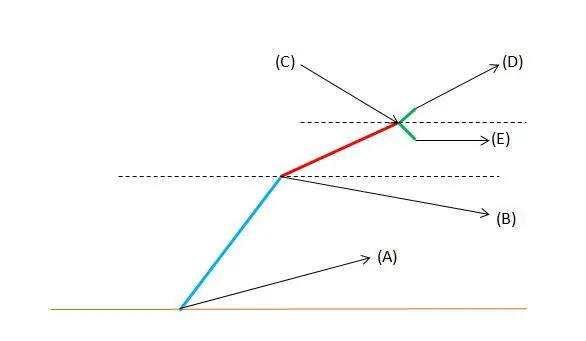
Figure 1
This kinematic chain is made up of a base, two kinematic links (robotic arms), & two rotating joints. And one manipulator is also attached at the end of link 2 as shown in figure 2. When these links are programmed, a motion will be incorporated into them.
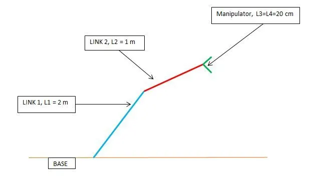
Figure 2
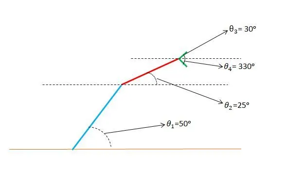
Figure 3
As shown in figure 3, link 1 is creating an angle with regard to the base, while link 2 is creating an angle with respect to link 1. And the manipulator is making & an angle. There is no revolute joint between link 2 and the manipulator. One revolute joint is between link 2 & link 1 and another is between link 1 & base which is fixed at the surface.
In order to design a plot where these arms can move at different angle points, we must ascertain the coordinates at the joints in order to perform this. So the coordinates will be `(x_0,y_0)` at point A, at point B `(x_1,y_1)`, at point C `(x_2,y_2)`, at the end of the manipulator i.e., points D & E are `(x_3,y_3)` and `(x_4,y_4)` respectively, as shown in figure 4.
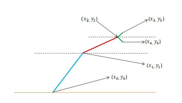
Figure 4
From figure, we find out some relations & values between linkages. And we are going to use all these information in our program.
Coordinates of robotic arm figure;
At point A, `(x_0,y_0)` = (0, 0)
At point B, `(x_1,y_1)` = (`l_1`*Cos`θ_1`, `l_1`*Sin`θ_1`)
At point C, `(x_2,y_2)` = (`x_1`+ (`l_2`*Cos`θ_2`)), ( `y_1`+ (`l_2`*Sin`θ_2`))
At point D, `(x_3,y_3)` = (`x_2`+ (`l_3`*Cos`θ_3`)), ( `y_2`+ (`l_3`*Sin`θ_3`))
At point E, `(x_4,y_4)` = (`x_2`+ (`l_4`*Cos`θ_4`)), ( `y_2`+ (`l_4`*Sin`θ_4`))
Positions of links;
From A to B = Link 1 `(l_1)`
From B to C = Link 2 `(l_2)`
From C to D = Link 3 `(l_3)`
From C to E = Link 4 `(l_4)`
Here we are going to make 3 programs;
In the first program, we are simply going to plot these kinematic arms for one position in the graph with the help of Matlab for the given inputs.
Inputs;
Length of Link 1 `(l_1)`= 1 m
Length of Link 2 `(l_2)`= 0.5 m
Length of Link 3 `(l_3)`= 0.1 m
Length of Link 4 `(l_4)`= 0.1 m
`θ_1`= 45ᵒ
`θ_2`= 0ᵒ
`θ_3`= 30ᵒ
`θ_4`= 330ᵒ
Before starting the coding, one should write a comment on the editors’ window and also write the clear all, close all & clc command, if you have executed any program before this program because by using these commands all previous data from the workspace would be removed, from this some system memory will be free and also deletes the current plot or the specified figure. Using the clc command clears all input & output from the Command Window, & giving you a clean screen.
After heading comment, we will write all the given inputs which are given for this program. Like the length of the link, given value of coordinates & equation for unknown coordinates with comments.
In this particular program, we are not using for end loop command, after this, we are directly going for a plot with the help of the line command in this program. With the help of this line command, we are going to plot a line between two coordinates. In this command, we are also going to define the width of the line and the color of the line. In this program line, A to B, B to C, C to D, and D to E are defined in blue, red, and green colors respectively.
After completing the writing process of the program, we will execute the program by pressing the F5 button or clicking on the icon (RUN).
If our program is written well, considering all the points which are important or necessary for the right execution of the program, will get correct results and plots. Otherwise, we will get an error on the command window. The program is written below and after execution, no error is found in the command window and Result is also attached below the program in the form of figure 5. By seeing the results one can say that program is correctly written.
% Program to plot the position of kinematics of Robotic Arm

% Input
% Length of links
l1 = 1;
l2 = 0.5;
l3 = 0.1;
l4 = 0.1;
% Angles
theta1 = 45;
theta2 = 0;
theta3 = 30;
theta4 = 330;

% Coordinates
x0 = 0;
y0 = 0;
x1 = l1*cosd(theta1);
y1 = l1*sind(theta1);
x2 = x1 + l2*cosd(theta2);
y2 = y1 + l2*sind(theta2);
x3 = x2 + l3*cosd(theta3);
y3 = y2 + l3*sind(theta3);
x4 = x2 + l3*cosd(theta4);
y4 = y2 + l3*sind(theta4);

% plotting
line([x0 x1],[y0 y1],'linewidth',3,'color','b')
line([x1 x2],[y1 y2],'linewidth',3,'color','r')
line([x2 x3],[y2 y3],'linewidth',3,'color','g')
line([x2 x4],[y2 y4],'linewidth',3,'color','g')
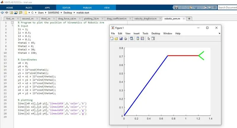
Figure 5
In the second program, we are going to plot these kinematic arms for different positions in the graph with the help of Matlab for the given inputs.
Inputs;
Length of Link 1 `(l_1)` = 1 m
Length of Link 2 `(l_2)` = 0.5 m
Length of Link 3 `(l_3)` = 0.1 m
Length of Link 4 `(l_4)` = 0.1 m
In this program, both `θ_1` & `θ_2`are defined by using the linspace command. It is a range operator and by this linearly spaced vectors will be generated. So in this case values of `θ_1`and `θ_2` will be between 0ᵒ to 90ᵒ including 0ᵒ & 90ᵒ. linspace(0,90,5) means that Matlab will generate a row vector of 5 points. linspace(0,90,4) means that Matlab will generate a row vector of 4 points.
`θ_1`= linspace(0,90,5)
`θ_2`= linspace(0,90,4)
`θ_3`= 30ᵒ
`θ_4` = 330ᵒ
In this program, we are going to use for loop command. It is a repetition control command that allows you to efficiently write a loop that needs to execute a specific number of times. Here `θ_1`and `θ_2`are contain multiple values of the angle within the program, so a new variable is needed inside the for loop command for both `θ_1` &`θ_2`. THETA 1 & THETA 2 are added to the code, for THETA 1 = `θ_1` (i) and THETA 2 = `θ_2` (j). Where i = 1:length(`θ_1`) & j = 1:length(`θ_2`). Here the length of `θ_1`is equal to 5 and the length of `θ_2`is equal to 4. And after this everything is the same as what we have done previously in the first program. The end command was used to plot the lines & to stop the for loop command. The program is written below and after execution, no error is found in the command window and Result is also attached below the program in the form of figure 6.
% Program to plot the position of the kinematics of Robotic Arm
% Input

% Length of links
l1 = 1;
l2 = 0.5;
l3 = 0.1;
l4 = 0.1;

% Angles
theta1 = linspace(0,90,5); % Five value of theta1
theta2 = linspace(0,90,4); % Four value of theta2
theta3 = 30;
theta4 = 330;

for i = 1:length(theta1) % Executing multiple values
    THETA1 = theta1(i);
    for j = 1:length(theta2)
        THETA2 = theta2(j);
% Coordinates
x0 = 0;
y0 = 0;
x1 = l1*cosd(THETA1);
y1 = l1*sind(THETA1);
x2 = x1 + l2*cosd(THETA2);
y2 = y1 + l2*sind(THETA2);
x3 = x2 + l3*cosd(theta3);
y3 = y2 + l3*sind(theta3);
x4 = x2 + l3*cosd(theta4);
y4 = y2 + l3*sind(theta4);

% plotting
line([x0 x1],[y0 y1],'linewidth',3,'color','b')
line([x1 x2],[y1 y2],'linewidth',3,'color','r')
line([x2 x3],[y2 y3],'linewidth',3,'color','g')
line([x2 x4],[y2 y4],'linewidth',3,'color','g')
    end
end
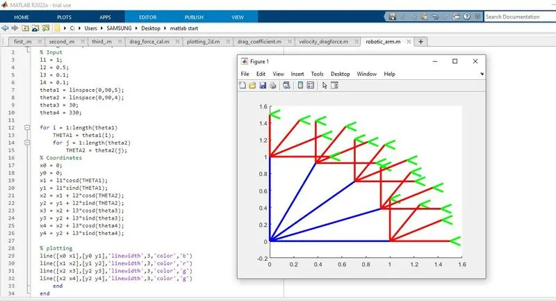
Figure 6
In the third program, we are going to plot these kinematic arms for different positions in the graph with the help of MatLab for the given inputs. And also going to make a single animation video of these entire plots.
Inputs;
Length of Link 1 `(l_1)` = 2 m
Length of Link 2 `(l_2)` = 1 m
Length of Link 3 `(l_3)` = 0.2 m
Length of Link 4 `(l_4)` = 0.2 m
In this program, both `θ_1` and `θ_2`are defined by using the linspace command. It is a range operator and by this linearly spaced vectors will be generated. So in this case values of `θ_1` andm`θ_2` will be between 0ᵒ to 150ᵒ & 0ᵒ to 75ᵒ, including 0ᵒ & 150ᵒ, 0ᵒ & 75ᵒ linspace(0,150,50) means that Matlab will generate a row vector of 50 points. linspace(0,75,25) means that Matlab will generate a row vector of 25 points.
`θ_1`= linspace(0,150,50)
`θ_2`= linspace(0,75,25)
`θ_3`= 30ᵒ
`θ_4`= 330ᵒ
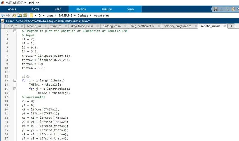
In this program, we are going to use for loop command. It is a repetition control command that allows you to efficiently write a loop that needs to execute a specific number of times. Here `θ_1`and `θ_2`are contain multiple values of the angle within the program, so a new variable is needed inside the for loop command for both `θ_1` & `θ_2`. THETA 1 & THETA 2 are added to the code, for THETA 1 = `θ_1`(i) and THETA 2 = `θ_2` (j). Where i = 1:length(`θ_1`) & j = 1:length(`θ_2`). Here the length of `θ_1` is equal to 50 and the length of `θ_2` is equal to 25. A pause command is used for pausing the command for a certain time, for this program will be paused for 0.01 seconds. The M command is used to capture the current frame, every time the for loop runs. In the last step of the loop, we have added a ct+1 to the ct variable; this will increment the value of the frame every time the for loop runs.
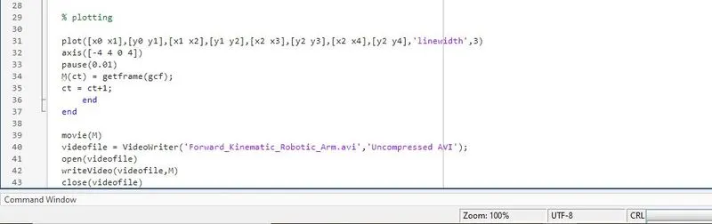
The end command is used to plot the lines & to stop the for loop command. In the last step of the program is to create a movie of the animation of the robotic arm, so the movie command is used; videofile defines the name and format of the video. VideoWriter command is used to define & assign the video format, for this project AVI is used as the format. The open command is used to open the video; writevideo command is used to write the video with plot frames. Finally, the close command is used to close the video file. The result is also attached below the program in the form of figure 7. And YOUTUBE's link is attached below the program.
% Program to plot the position of kinematics of Robotic Arm
% Input
% Length of links
l1 = 2;
l2 = 1;
l3 = 0.2;
l4 = 0.2;
% Angles
theta1 = linspace(0,150,50); % Fifty values of theta1
theta2 = linspace(0,75,25); % Twenty five values of theta2
theta3 = 30;
theta4 = 330;

ct=1;
for i = 1:length(theta1) % Executing multiple values
    THETA1 = theta1(i);
    for j = 1:length(theta2)
        THETA2 = theta2(j);
% Coordinates
x0 = 0;
y0 = 0;
x1 = l1*cosd(THETA1);
y1 = l1*sind(THETA1);
x2 = x1 + l2*cosd(THETA2);
y2 = y1 + l2*sind(THETA2);
x3 = x2 + l3*cosd(theta3);
y3 = y2 + l3*sind(theta3);
x4 = x2 + l3*cosd(theta4);
y4 = y2 + l3*sind(theta4);

% plotting

plot([x0 x1],[y0 y1],[x1 x2],[y1 y2],[x2 x3],[y2 y3],[x2 x4],[y2 y4],'linewidth',3)
axis([-4 4 0 4])
pause(0.01) % Time in seconds
M(ct) = getframe(gcf);
ct = ct+1;
    end
end

% Commands of annimation
movie(M)
videofile = VideoWriter('Forward_Kinematic_Robotic_Arm.avi','Uncompressed AVI');
open(videofile)
writeVideo(videofile,M)
close(videofile)
Results
The final Animation of this MatLab program is uploaded on YouTube and can be seen by clicking on the given link below.