Week 9 - FVM Literature Review

Aim:

To describe finite volume methods, differences between finite volume and finite difference methods along with the need for the interpolation schemes in the FVM and flux limiter.

METHOD OF computational fluid dynamics:

To solve the real-world problems, three simples schemes for the numerical solution are employed which are

• Finite Difference Method
• Finite Element Method
• Finite volume Method

Finite Difference Method:

This method solves the equation, that is divided into single points or nodes. This method involves solving the discretizations using the differencing equation.

Finite Element Method:

This method involves dividing the domain into elements as desired, by solving the elements of the system. The finite element analysis is a particular method for solving two or three-dimensional problems.

Finite Volume Method:

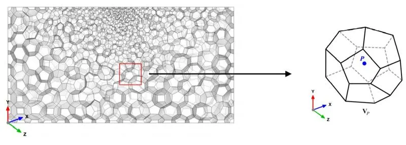
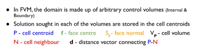
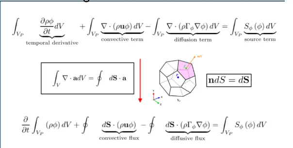
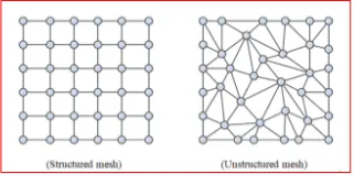
In the FVM Method the system is divided into an unstructured mesh which is conservative. In the algebraic form, the partial equation represents the volume integral, which is converted into the surface integral by the Gauss divergence theorem. These terms are solved as a flux on each surface. Because the flux entering the surface is identical to the adjacent surface, this is a conservative principle.

Gauss Divergence Theorem

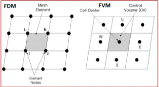
Differences between Finite Volume and Finite Difference approaches

S.no	Finite Volume Methods	Finite Difference methods
1	Governing equations are in the differential form.	Governing equations are in the integral form.
2	Solutions computed at each node i.e., intersectionof mesh lines.	Solution computed at the cell centroids.
3	Requires the usage of structured grid and hence diificult to implement for complex geometries.	Can handle unstructured grid and hence complex geometries with ease.
4	Easier to obtain higher order schemes this is preferable for applications requiring very high accuracy.	Deriving schemes higher than the second order is next to impossible due to the complexity involved.
5	All flow variables need to differentiable and continuous over the entire domain and hence not suited for handling discontinuities.	Can handle discontinuities due to the nature of integral equations.
6	Does not ensure conservation.	Imposes and ensures conservation at both cell and domain levels.

Application of finite volume method to 1-D steady-state heat conduction problem

The governing equation for one-dimensional steady-state heat conduction equation with source term is given as

`d/(dx) ( alpha ∗ (dT)/(dx)) + S = 0`

where 'T' is the temperature of the rod. The boundary values of temperature at A and B are prescribed.

`alpha` is thermal diffusivity.

S is the source term.

Grid generation

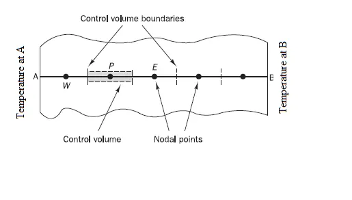
The first step in the finite control volume is to discretize the domain into discrete control volumes as shown in figure

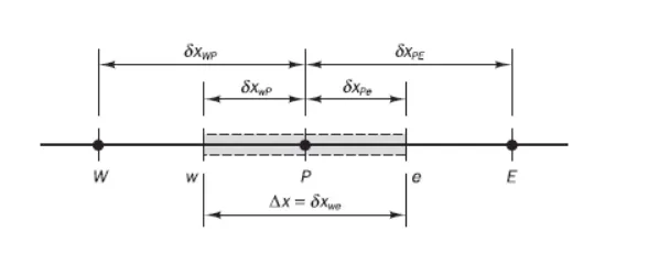
The number of nodal points is placed between A & B. The boundary of the control volume is positioned midway between the two adjacent nodes, thus each node is surrounded by the control volume. The control volume should be set up near the edges of the domain such that the physical boundary and the control volume boundary should coincide with each other.

A general nodal point is identified as P and its neighboring nodes to the west and east are identified as W and E respectively. The west side of the control volume is identified as w whereas the east side is identified as e. The distance between the nodes W and P, and between nodes P and E are identified as `delta x_(WP)` and `delta x_(PE)`respectively. Similarly between w and P, and between P and e are identified as `delta x_(wP)` and `delta x_(Pe)` . The control volume width is `Delta x = delta x_(we)`.

Discretization

The key step in the finite volume method is to integrate the governing equation over a control volume to yield a discretize equation at its nodal point P. For the control volume defined above this gives

`int_ (Delta V) d/(dx) ( α ∗ (dT)/ (dx)) ∗ d V + int_ (Delta V) SdV = 0`

`dV = A**dx`

The equation becomes

`(alpha ∗ A ∗ (dT)/ (dx)) e − (alpha ∗ A ∗ (dT)/ (dx)) w + S Delta V = 0`

A is the cross sectional area of the control volume.

`Delta V`s the control volume.

S is the average value of the source S over the control volume.

The above equation states that the diffusive flux of temperature leaving the east face of the control volume minus the diffusive flux of temperature entering the west face is equal to the generation of temperature. It constitutes a balance equation of temperature over a control volume.

In order to derive useful forms of the discretized equation, the interface diffusion coefficient `alpha` and temperature gradient `(dT)/ (dx)` at east and west face are required`. Linear approximations seem to be the obvious and simplest way of calculating interface values and gradients. This practice is called a central differencing scheme.

`alpha_ w = (alpha_ W + alpha_ P)/ 2`

`alpha_ e = (alpha_ E + alpha_ P)/2`

And the diffusive flux terms are evaluated as

`(alpha ∗ A ∗ (dT)/ (dx)) _e = alpha_ e ∗ A_ e ∗ (T_ E − T_ P) / (delta x _ (PE))`

`(alpha ∗ A ∗ (dT)/ (dx)) _w = alpha_ w ∗ A_ w ∗ (T_ P − T_ W)/ (delta x_ (W P))`

The finite volume method approximates the source term as

`S ∗ Delta V = S_ u + S_ p ∗ T_ P`

The final equation can be rearranged as

`(alpha_ e ∗ A_ e ∗ (T_ E − T_ P)/ (delta x_ (PE))) − ( alpha_ w ∗ A_ w ∗ (T_ P − T_ W)/ (delta x_ (WP))) + (S_ u + S_ p ∗ T_ P) = 0`

This can be arranged as

`((alpha_ e ∗ A_ e)/ (delta x_ (PE)) + (alpha_ w ∗ A_ w)/ (delta x_ (WP)) − S_ p) ∗ T_ P = ((alpha_ w ∗ A_ w)/ (delta x_ (WP))) ∗ T_ W + ((alpha_ e ∗ A_ e)/ (delta x_ (PE))) ∗ T_ E + S_ u`

Identifying the coefficient of `T_P`,`T_W`,`T_E`TP,TW,TE">, as `alpha_ W`,`alpha_ P`,`alpha_E`and rearranging the equation as under

`a_ P ∗ T_ P = a_ W ∗ T_ W + a_ E ∗ T_ E + S_ u`

where,

Interpolation schemes

The approximation of the surface and volume integrals may require values of the variable at locations other than the computational nodes of the control volume (CV). Values at this location are obtained using interpolation formulae.

The interpolation schemes are listed below

• First-order upwind scheme

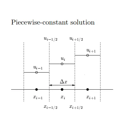
Upwind biased interface values

`v>0`

`u_ (i − 0.5) ≈ u_ (i − 1)`

`u_ (i + 0.5) ≈ u_ i`

Backward differencing

`I_ c = v ∗ (u_ i − u_ (i − 1))/ (dx)`

Forward differencing

`v<0`

`u_ (i − 0.5) ≈ u_ i`

`u_ (i + 0.5) ≈ u_ (i + 1)`

`I_ c = v ∗ (u_ (i + 1) − u_ i)/ (dx)`

Taylor series expansion

`v u_ (i+0.5) = v u_ i + (v Delta x)/ 2 ⋅ ((del u)/ (del x)) _ (i + 0.5) + (v (Delta x) ^ 2)/ 8 ⋅ ((del^2 u)/ (del x^ 2)) _ (i+ 0.5) + ....`

a first order accurate flux approximation, the leading truncation error resembles a diffusive flux `d (del u)/(del x)` with `d = (v Delta x)/2`being the numerical diffusion coefficient.

• Central difference approximation

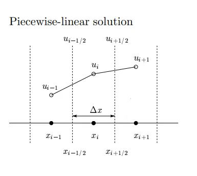
Interpolation polynomial

`p_1 (x) = u_ L (x_ R − x)/ (x_ R − x_ L) + u_ R (x − x_ L)/ (x_ R − x_ L)`

Average interface values

`u_ (i − 0.5) ≈ (u_ (i − 1) + u_ i)/ 2, u_ (i+0.5) ≈ (u_ i + u_ (i+1))/ 2`

`I_ c = v (u_ (i+1) − u_ (i−1))/ (2 Delta x)`

`u_ (i+1) = u_ (i+0.5) + (Delta x)/2 ∗ ((del u)/ (del x)) _(i+0.5) + (Delta x) ^ 2/ 8 ((del^ 2 u)/ (del x^ 2)) _ (i+0.5) + ... ...`

`u _i = u_ (i + 0.5) − (Delta x)/ 2 ∗ ((del u)/ (del x)) _ (i+0.5) + (Delta x) ^ 2/ 8 ((del^2 u)/ (del x^ 2)) _ (i+0.5) + ... ...`

`u_ (i+0.5) = (u_ i + u_ (i+1))/2 − (Delta x) ^ 2/ 8 ⋅ ((del^2 u)/ (del x ^2)) _ (i+0.5)` (second-order accuracy)

• Quadratic upwind difference scheme (QUICK)

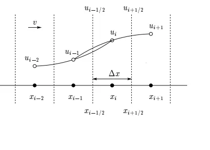
Quadratic upwind interpolation for convective kinematics

`p_2 (x) = u_ L (x − x_ M)/ (x_ L − x_ M) (x_ R − x)/ (x_ R − x_ L) + u_ M (x − x_ L)/ (x_ M − x_ L) (x_ R − x)/ (x_ R − x_ M) + u_ R (x − x_ L)/ (x_ R − x_ L) (x − x_ M)/ (x_ R − x_ M)`

Upwind biased interface values

`v>0`

`u_ (i−0.5) ≈ (3 u_ i+ 6 u_ (i−1) − u_ (i−2))/ 8`

`u_ (i+0.5) ≈ (3 u_ (i+1) + 6 u_ i − u_ (i−1))/ 8`

`I_ c ≈ v (3 u_ (i+1) − 7 u_ (i−1) + 3 u_ i + u_ (i−2))/ (8 Delta x)`

`v < 0`

`u_ (i−0.5) ≈ (3 u_ (i−1) + 6 u_ i − u_ (i+1))/ 8`

`u_ (i+0.5) ≈ (3 u_ i + 6 u_ (i+1) − u_ (i+2))/ 8`

`I_ c ≈ − v (3 u_ (i−1) − 7 u_ (i+1) + 3 u_ i + u_ (i+2))/ (8 Delta x)`

• Third order flux approximation.
• Second-order overall accuracy (because of the midpoint rule).

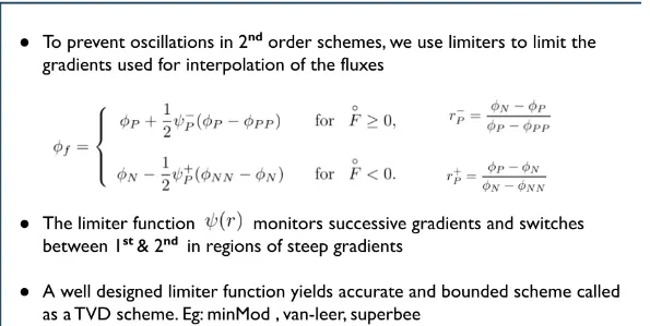
Flux limiters

They are used in high-resolution schemes to avoid spurious oscillations (wiggles) that would otherwise occur with high-order spatial discretization schemes due to shocks, discontinuities, or sharp changes in the solution domain. For smoothly changing solution flux limiters are not used and the spatial derivatives can be implemented with high-resolution schemes. If there are discontinuities in the domain the fux limiters change the solution to low and high-resolution schemes depending upon the gradients in the nearby surroundings.

Case-1

Absence of source term in the heat conduction equation

`d/ (dx) (K ∗ (dT)/ (dx)) = 0`

Integrating above the control volume `dV`

`(2∗K∗A)/ (dx) ∗ T_ P = (K∗ A)/ (dx) ∗ T_ A + (K ⋅ A)/ (dx) ∗ T_E + q∗ A∗ dx`

And discretization of the above equation will yield

`K ⋅ A ⋅ ((T_ E − T_ P)/ (dx)) − K ⋅ A ⋅ ((T_P − T_W)/ (dx)) = 0`

`(2∗ K∗ A)/ (dx) ∗ T_P = (K∗ A)/ (dx) ∗ T_ E + (K ⋅ A)/ (dx) ∗ T_ W`

The above equation represents the solution of temperature at the inner nodes.

The node associated with the left boundary

`(2∗ K∗ A)/ (dx) ∗ T_ P = (K ∗ A)/ (dx) ∗ T_ A + (K⋅ A)/ (dx) ∗ T_ E`

The node associated with the right boundary

`(2∗ K∗ A)/ (dx) ∗ T_ P = (K∗ A)/ (dx) ∗ T_ B + (K ⋅ A)/ (dx) ∗ T_ W`

Case-2

Presence of source term in the heat conduction equation

`d/ (dx) (K ∗ (dT)/ (dx)) + q = 0`

`(2∗ K∗ A)/ (dx) ∗ T_ P = (K∗ A)/ (dx) ∗ T_ E + (K⋅ A)/ (dx) ∗ T_ W + q ∗ A ∗ d x`

The above equation represents the solution of temperature at the inner nodes.

The node associated with the left boundary

The node associated with the right boundary

`(2 ∗ K ∗ A)/ (dx) ∗ T_ P = (K∗ A)/ (dx) ∗ T_ B + (K ⋅ A)/ (dx) ∗ T_ W + q ∗ A ∗ d x`