Week 3 - Solving second order ODEs

Aim:-

To solve the ODE which represents the equation of motion of a simple pendulum.

objective:-

To write a program that solves the ODE which represents the equation of motion of a simple pendulum with damping and create an animated video of output obtains by solving this ODE.

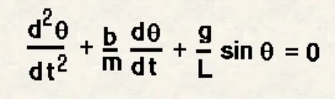
Where,

g = gravity in m/s^2.

L = length of the pendulum in the meter.

m = mass of the ball inn kg.

b = damping coefficient.

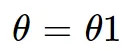
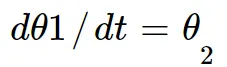
since the given function is in the second-order differential equation we will convert it into first order to solve the ODE.

Let

Inputs:

L = 1 meter

m = 1 kg

b = 0.05

g = 9.81 m/s^2

Time span =0-20 sec

angular displacement = 0

angular velocity = 3 rad/sec^2 at time t = 0

Theory:-

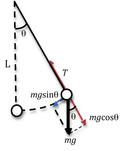
The motion of a simple pendulum is a basic classical example of simple hormonic motion,consisting of a small bob and a massless string. Movement of the pendulum depends on Newton's second law. A second-order Ordinary Differential Equation is formed that describes the position of the end of the pendulum with respect to time.

Main code:

% Second order ODE program
close all
clear all
clc

b = 0.05;
g = 9.81;
l = 1;
m = 1;

% Initial condition
theta_0 = [0;5];

% Time  points
t_span =  linspace(0,20,500);

% solve ODE equation
[t, results] = ode45(@(t,theta)ode_func(t,theta,b,g,l,m),t_span,theta_0);

% Plotting 
figure(1)
plot(t,results(:,1))
hold on
plot(t, results(:,2))
xlabel('Time')
ylabel('Plot')

disp = results(:,1);
ct = 1;
for i =1:length(t_span)

    x0 = 0;
    y0 = 0;

    x1 = l*sin(disp(i));
    y1 = -l*cos(disp(i));

    figure(2)
    plot([-2 2],[0 0], 'LineWidth',5)
    hold on
    plot([x0 x1], [y0 y1], '-O','MarkerSize',3,'LineWidth',3,'Color','y');
    plot(x1, y1, '-O', 'MarkerSize',15,'MarkerFaceColor','r');
    axis([-1.5 1.5 -1.5 1.5])
    pause(0.03)
    hold off
    M(ct) = getframe(gcf)

    ct = ct+1


end

movie(M);
videofile = VideoWriter('Pendulum.avi','Uncompressed AVI');
open(videofile);
writeVideo(videofile,M);
close(videofile);

function [dtheta_dt] = ode_func(t, theta, b, g, l, m)

theta1 = theta(1)
theta2 = theta(2)
dtheta1_dt = theta2;
dtheta2_dt = -(b/m)*theta2 - (g/l)*sin(theta1);
dtheta_dt = [dtheta1_dt; dtheta2_dt];
end

Output:

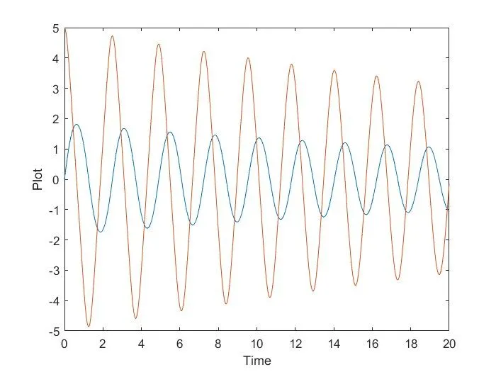
The output obtained is graphical representation velocity curve and displacement curve W.r.t Time.

Angular Displacement and Angular Velocity plots were generated for a time range of 20 secs.

Video Link : https://drive.google.com/file/d/1KV6LccVIb5tgg5JOAr1T5GINB4deJ36T/view?usp=sharing