Week 9 - FVM Literature Review
Introduction
Finite Volume Method(FVM) :- Finite volume method (FVM) is a method of solving the partial differential equations in the form of algebraic equations at discrete points in the domain. Similar to finite difference methods, the finite volume method (FVM) solves partial differential equations as algebraic equations at discrete points in the domain.The finite volume method is evaluated at the volume surrounding the nodes, whereas the finite difference method is evaluated at the nodes themselves.The partial differential equation is integrated over the small volume in the finite volume method.The Gauss Divergence Theorem is used to transform a volume integral with a divergence term into a surface integral.The fluxes at the finite volume's surfaces are used to evaluate these surface integrals.The finite volume method is conservative because the flux entering a control volume should be the same as the flux leaving an adjacent control volume.Apart from its simplicity, the fact that the conservation of properties is applicable across any finite control volume makes the finite volume method suitable for use with unstructured meshes.Although the unstructured mesh must be transformed via linear transformation into a structured mesh (cartesian mesh) before the finite difference scheme can be used, this requires more computational resources.In the case of moving meshes, this is extremely undesirable. It is always better to use governing equation in conservative form with finite volume approach to solve any problem which ensures conservation of all the properties in each cells/control volume. One advantage of the finite volume method over finite difference methods is that it does not require a structured mesh (although a structured mesh can also be used).
| Finite Difference Method (FDM) |
Finite Volume Method (FVM) |
| The method is approximated by Taylor series. | The finite element method (FEM) is a popular method for numerically solving differential equations. |
| It is evaluated at nodes. | It is evaluated at the volume surrounding by the nodes. |
| Uses regular grid. | Can use irregular grids |
| Low memory requirement. | Larger memory requirement. |
| It is highle undesirable in the case of moving meshes. | It is desirable in the case of moving meshes. |
TYPES OF FINITE VOLUME GRIDS
1. Cell centred approach: Control volumes are defined by a suitable grid and computational nodes are assigned at the Control volume centre. It can be applied for both structured and unstructured grids. This approach is the most commonly used in the Finite volume Method.
2. Face centred approach: Nodal locations are defined first and control volumes are then constructed around them so that the control volume faces lie in the midway between the nodes. It can only be used with structured grids.
Example of Finite Volume Method TO 1-D LINEAR HEAT CONDUCTION EQUATION Problem:
The governing equation for 1 dimensional steady heat conduction is `d/dx(k(dT)/dx)+S = 0`
where, T = temperature of rod
k = thermal conductivity
S = source term.
Now we shall discuss the steps involving FVM for solving differential equation:
Step 1 : Grid Generation
The first step in the finite volume method is grid generation by dividing the domain in to discrete control volumes. Let us place a number of nodal points in the space between A and B. The boundaries of control volumes are positioned mid-way between adjacent nodes. Thus each node is surrounded by a control volume or cell.
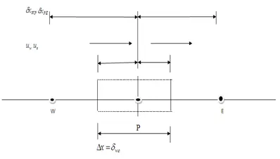
The shaded area represents the finite control volume and the capital letter P denotes the control volume's center if we are evaluating the equation at node 2.The centers of control volumes to the left (west) and right (east) of the control volume under evaluation are denoted, respectively, by the capital letters W and E.The interface between W P E and P E is denoted by the small letters w and e, respectively.
We have assumed a uniform grid for this problem, where x is the size of the grid.Now, the differential equation is integrated over the control volume as follows:
Step 2 : Discretization
The most important features of finite volume method are the integration of the governing equation over a control volume to yield a discretized equation to yield a discretized equation at its nodal points P.
`int_{Delta V} d/dx(K{dT}/dx)dV + int_{Delta V} S dV = 0`
`dV=A*dx` and `Delta V = Adelta x`
So, the equation becomes
`int_w^e d/dx(kA{dT}/dx)dx + (S)int_{Delta V}dV = 0`
`(KAfrac{dT}{dx})_e-(KAfrac{dT}{dx})_w+StriangleV=0`
A = is the cross sectional area
The above equation states that the diffusive flux of temperature leaving the east face of the control volume minus the diffusive flux of temperature entering the west face is equal to the generation of temperature.
INTERPOLATION SCHEMES
We need to use some interpolation schemes to estimate the values through the nodal values in order to evaluate the temperature values and temperature gradients at the interfaces.Similar Taylor series expansions are used to evaluate differentials in finite difference methods, these interpolation schemes evaluate differentials at interfaces rather than nodes in this case. There are different interpolation schemes of various orders as follows:
1. First-order upwind scheme
The first-order upwind scheme is used to discretize the convection term in the momentum and energy equations. In this method, we assume that the value at the interface is the same as the value at the center of the control volume depending on the direction of the flow. The first order upwind scheme considers one upstream point . The first order scheme is easier to converge but less accurate.
2. Second order upwind scheme
In this scheme, the value of the flux at the interface is determined from two points upstream of the transport direction rather than equal to the first point upstream. Second order upwind scheme considers two points. The second order is difficult to converge but more accurate.
3. Quadratic upwind interpolation for convective kinetics (QUICK) scheme
QUICK, which stands for Quadratic Upstream Interpolation for Convective Kinematics, is a higher order differencing scheme that considers a three-point upstream weighted quadratic interpolation for the cell face values. When solving convection–diffusion equations, this method used a second-order central difference for the diffusion term and is third-order accurate in space and first-order accurate in time for the convection term. This scheme is most appropriate for steady flow.
4. Central Differencing Scheme
The central differencing scheme is used to optimize the approximation for the differential operator in the central node of the considered patch and provides numerical solutions to differential equations. This scheme is a second order scheme and is thus more accurate than the first order scheme.
cell face values of property for a uniform grid can be written as
`phi_e = (phi_E + phi_P)/2`
`phi_w = (phi_W + phi_P)/2`
Flux limiters
Flux limiters are used in high resolution schems – numerical schemes used to solve problems in science and engineering, mainly fluid dynamics , described by Partial differential equations (PDEs). High resolution scheme is used in the numerical solutions of the partial differential equations where high accuracy is required. The main idea behind the construction of flux limiter schemes is to limit the spatial derivatives to realistic values. Flux limiter don't let the solution value to overshoot.
References:
1.A. Shukla, A. Singh, and P. Singh, A Comparative Study of Finite Volume Method and Finite Difference Method for Convection-Diffusion Problem