Week 4.1 - Genetic Algorithm

Title :GENETIC ALGORITHM

AIM: TO OPTIMIZE THE STALAGMITE FUNCTION AND CALCULATE THE GLOBAL MAXIMA OF THE STALAGMITE FUNCTION USING MATLAB

Genetic Algorithm : The genetic algorithm is a method for solving both constrained and unconstrained optimization problems that is based on natural selection, the process that drives biological evolution.

The main processes going behind the GA is

1.Selection

2.Crossover

3.Mutation

First of all Genetic algorithm will crate a random initial population and they will give rise the next generation by computing its fitness value.Replaces the current population to form the next generation and this process repeats itself until it gets the optimal value.

Explanation the syntax for ga in matlab :

x = ga (fun, nvars, A, b, Aeq, beq, lb, ub, nonlcon, options)

fun = Objective function (In our problem stalagmite function is the objective function)

nvar = Number of Variables (specified as positive integer, in our problem its x,y)

A,b = Linear inequality constraints ( A = Real matrix; b = Real vector)(In our problem there is no condition , thats why we have put the empty bracket in that place)

Aeq,beq = Linear equality constraints (A = Real matrix; b = Real vector)(Its also empty ,in our case)

Lb,ub = Lower bounds and upper bounds( In our problem for case 2 and case 3 , lower bounds is [0;0] and upper bounds is [0.4;0.4])

nonlcon = Nonlinear constraints (Its also absent in our case ,that why we used [] empty bracket)

options = Optimization options (optimoptions is used to define the population size.)

Applied Equation :

`f1x = (sin((5.1*pi*x)+0.5))^6`

`f1y = (sin((5.1*pi*y)+0.5))^6`

`f2x = exp(-4*log(2)*((x-0.0667)^2)/0.64))`

`f2y = exp(-4*log(2)*((y-0.0667)^2)/0.64))`

stalagmite function , `f = -(f1x*f1y*f2x*f2y)`

Main code:

clear all
close all
clc

% Defining the inputs
x = linspace(0,0.6,150);
y = linspace(0,0.6,150);

%% Evaluating the objective function
% Creating a 2D mesh
[xx, yy] = meshgrid(x, y); 

% Asiigning values to inputs
for i = 1:length(x)
    for j = 1:length(y)
        inputs (1) = xx(i , j);
        inputs (2) = yy(i , j);
        f(i,j) = stalagmite(inputs);
    end
end

num_case = 50;
%% Case 1 Unbounded GA study

for z = 1:num_case
    [inputs,fopt(z)] = ga(@stalagmite,2);
    xopt(z) = inputs (1);
    yopt(z) = inputs (2);
end

figure(1)
subplot(2,1,1)
surfc(xx,yy,-f)
hold on

% For Removing the gridlines on the 3D surface plot
shading interp

plot3(xopt,yopt,-fopt,'marker','*','markersize',3)
title('Case 1 Unbounded ')
subplot(2,1,2)
plot(-fopt)
xlabel('Number of iterations')
ylabel('F maximum')


%% Cae 2 Bounded GA study

for z = 1:num_case
    [inputs,fopt(z)] = ga(@stalagmite,2,[],[],[],[],[0;0],[0.4;0.4]); % Defines a set of lb and Ub 
    xopt(z) = inputs (1);
    yopt(z) = inputs (2);
end

figure(2)
subplot(2,1,1)
surfc(xx,yy,-f)
hold on

% For Removing the gridlines on the 3D surface plot
shading interp

plot3(xopt,yopt,-fopt,'marker','*','markersize',3)
title('Case 2 Bounded GA ')
subplot(2,1,2)
plot(-fopt)
xlabel('Number of iterations')
ylabel('F maximum')


%% Case 3 Bounded GA study with population size

options = optimoptions('ga')
options = optimoptions(options,'PopulationSize',270); % Defining the population size

for z = 1:num_case
    [inputs , fopt(z)] = ga(@stalagmite,2,[],[],[],[],[0;0],[0.4;0.4],[],[],options)
    xopt(z) = inputs (1)
    yopt(z) = inputs (2)
end

figure(3)
subplot(2,1,1)
surfc(xx,yy,-f)
hold on

% For Removing the gridlines on the 3D surface plot
shading interp

plot3(xopt,yopt,-fopt,'marker','*','markersize',3)
title('Case 3 Bounded GA with population size')
subplot(2,1,2)
plot(-fopt)
xlabel('Number of iterations')
ylabel('F maximum')

Function code for stalagmite :

function [f] = stalagmite(V)
x = V(1);
y = V(2);

first_term = (sin((5.1*pi*x)+0.5))^6;
second_term = (sin((5.1*pi*y)+0.5))^6;
third_term = exp(-4*log(2)*(((x-0.0667)^2)/0.64));
fourth_term = exp(-4*log(2)*(((y-0.0667)^2)/0.64));

f = -(first_term*second_term*third_term*fourth_term);
end

Explanation of the code :

STUDY 1: - The first study concerns with the unbounded inputs provided for calculating the value of Global Maxima. As it is unbounded, so we have used only stalagmite function and the number inputs variables. In our case the number of input variables are 2(x,y) and plot the x,y,z using the plot3 command and surfc.

Study 2: - The second study concerns with the bounded inputs provided for calculating the value of Global Maxima.Here the lower bound is [0;0] and upper bound is [0.4;0.4]. And empty bracket for the absent of linear constraint and plot the figure 2.

Study 3: - The third study concerns with the bounded inputs provided but with a population size for better optimization in order to calculate the value of Global Maxima. In order to defining the population size we have used the in-buit command of Matlab optimoptions.

Results /Outputs:

Study 1:

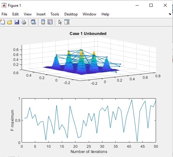
It can be observed that the value of F Maximum lies between the interval [0,1].Second case can give more good result.

Study 2 :-

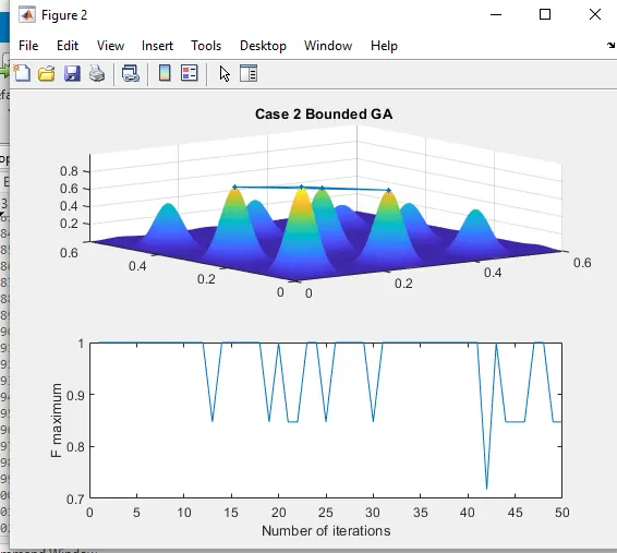
Foe For better result, we can specify the population size and will look for study 3.

Study 3:-

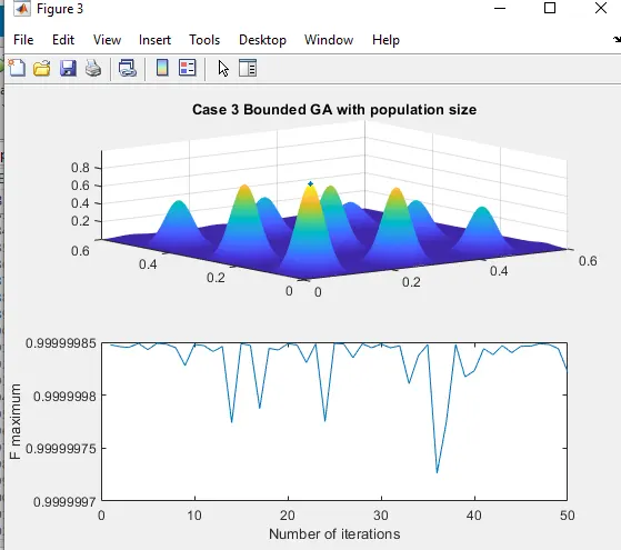
Assumed value of pulation size is 270. It has given us the more accurate value of the global maxima.

The value of global maxima is 0.99999985 got from the study 3.

Worskpace and command window screenshot:

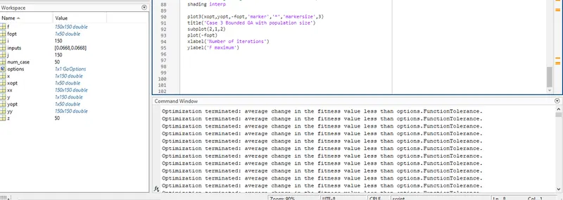
Conclusion :- The golbal maxima is calculated by defining the population size and the plots provided the visual context of solution with the interval.

References :- Mathworks,

Quora ,

https://skill-lync.com/knowledgebase/genetic-algorithm-explained