Week 9 - FVM Literature Review

FINITE VOLUME METHOD

AIM:

To Explain in detail about Finite Volume Method (FVM) and also to describe the need for Interpolation Schemes and Flux limiters in Finite Volume Method.

OBJECTIVE:

• To describe about Finite Volume Method (FVM) in detail.
• To distinguish between Finite Volume Method (FVM) and Finite Difference Method (FDM).
• To describe need for various interpolation schemes in Finite Volume Method (FVM).
• To elobrate the term Flux Limiters in FVM.

INTRODUCTION:

DISCRETIZATION:

Discretization methods are used to divide the region of a continuous function i.e., the real solution to a system of differential equations into a discrete function, where the solution values are defined at each point in space and time. Discretization simply refers to the spacing between each point in solution space and then replace derivatives in the governing equation with difference quotients.

FINITE DIFFERENCE METHOD:

In numerical analysis, finite-difference methods (FDM) are a class of numerical techniques for solving differential equations by approximating derivatives with finite differences. Based on finite differences, it gives the numerical solutions for the values at discrete points in the domain which are known as grid points.

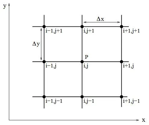
Finite differences method are used to compute approximate derivatives. This is used in numerical analysis in numerical ordinary differential equations and numerical partial differential equations, which gives the numerical solution of ordinary and partial differential equations respectively. The resulting methods are called finite-difference methods. Finite difference representations of derivatives are derived from Taylor series expansions.

FINITE VOLUME METHOD:

The finite volume method (FVM) is a discretization technique for partial differential equations. FVM uses a volume integral formulation of the problem with a finite partitioning set of volumes to discretize the equations.

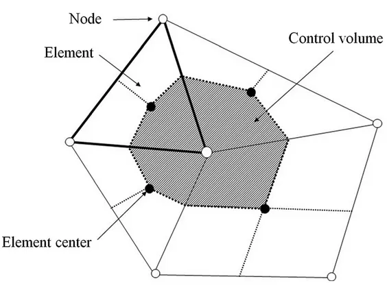
In the finite volume method, volume integrals in a partial differential equation that contain a divergence term are converted to surface integrals, using the divergence theorem. These terms are then evaluated as fluxes at the surfaces of each finite volume. Because the flux entering a given volume is identical to that leaving the adjacent volume, these methods are conservative.

DIVERGENCE THEOREM:

The divergence theorem states that the surface integral of a vector field over a closed surface, which is called the "flux" through the surface, is equal to the volume integral of the divergence over the region inside the surface. Intuitively, it states that "the sum of all sources of the field in a region with sinks regarded as negative sources gives the net flux out of the region.

The divergence theorem is employed in any conservation law which states that the total volume of all sinks and sources, that is the volume integral of the divergence, is equal to the net flow across the volume's boundary

`intintint_v(grad.F).dV= intint_s(F.n).ds`

The left side is a volume integral over the volume V, the right side is the surface integral over the boundary of the volume V.

MAJOR DIFFERENCE BETWEEN FINITE VOLUME METHOD (FVM) AND FINITE DIFFERENCE METHOD (FDM):

• The finite-difference method is the most direct approach to discretizing partial differential equations. By considering a point in space continuum representation of the equations and replace it with a set of discrete equations, called finite-difference equations. The finite-volume method is based on the fact that many physical laws are conservation laws—what goes into one cell on one side needs to leave the same cell on another side.
• The finite-difference method is defined dimension per dimension; this makes it easy to increase the “element order” to get higher-order accuracy.
• The finite-volume method’s strength is that it only needs to do flux evaluation for the cell boundaries. This also holds for nonlinear problems, which makes it extra powerful for robust handling of (nonlinear) conservation laws appearing in transport problems.
• In Finite Difference Method Approximate and replace all the derivatives by their corresponding finite difference approximations and Solve the resulting algebraic system of equations.
• In Finite Volume Method Discretize the integral conservation equation on control volumes and Solve the resultant discrete integral/flux equations.

EXAMPLE:

Consider a 1 Dimensional steady state heat conduction equation with heat generation,

`del/(del x).(alpha .((delT)/(del x))+s=0`

Where,

S is the source term

If small control volume dv is considered and it is multiplied with the governing equation and integrated for entire volume then that should be also equal to zero i,e the Integral form of governing equation.

Multiplying the equation with dv and integrating it,

`int(del/(del x).(alpha .((delT)/(del x))+s).dv=0`

dv= A.dx

`int(del/(del x).(alpha .((delT)/(del x)).A.dx+s.dv=0`

`[alpha.A.((del T)/(del x))]_w^e +s.dv=0`

S is the average value os source term(S) which when multiplied by dv is going to be equal to,

`s_Linearization --> s_u +s_pT_p Also Assuming Alpha as a constant and not a function of temperature.

`alpha .A.[(T_e-T_p)/(delx)]-alpha .A.[(T_p-T_w)/(delx)] +s.dv=0`

`[Heat Flux]_(out)-[Heat Flux]_((In)+SourceTerm=0

INTERPOLATION SCHEMS IN FINITE VOLUME METHOD (FVM):

Finite-volume methods require values (and derivatives) of various variables at the cell faces, when they are originally only known at the cell centers. The flow direction is often considered when these quantities are determined for convective terms. Time derivatives are also numerically approximated.

Interpolation is a process to estimate the values at unknown points by using the points with known value and sample points on either sides of the unknown point. In FVM, interpolation schemes are used to find values of volume integrals required at the points other than nodes.

THE DIFFERENT INTERPOLATION SCHEMES:

• Upwind Interpolation Scheme (UDS)
• Linear Interpolation Scheme
• Quadratic Upwind Interpolation Scheme
• Hybrid Interpolation Scheme
• Total variation Diminishing Scheme
• Essentially Non-oscillatory interpolation Scheme

UPWIND INTERPOLATION SCHEME:

The upwind interpolation scheme (UDS) for approximating the value of a variable f at the east face of a control volume is given by,

`f_e= {(f_(p ) if (v.n)_e>0),(f_E if (v.n)_e<0)}` It is generally used convection dominated problems (i.e pe >1).

The values of the interface is given by:

For v > 0, we have,

Backward Difference,

`u_(i-1/2) approx u_(i-1) , u_(i+1/2) approx u_(i)`

`I_c approx v {u_i - u_(i-1)}/{Deltax}`

For v < 0, we have,

Forward Difference,

`u_(i-1/2) approx u_(i) , u_(i+1/2) approx u_(i+1)`

`I_c approx v {u_(i+1) - u_i}/{Deltax}`

By Taylor series expansion,

`vu_(i+1/2) = vu_i - {vDeltax}/2({delu}/{delx})_(i+1/2) - v(Deltax)^2/8({del^2u}/{delx^2})_(i+1/2) +.....`

A first order accurate flux approximation, the leading truncation error resembles a diffusive flux, `d{delu}/{delx}` with `d = {vDeltax}/2` being numerical diffusion coefficient.

LINEAR INTERPOLATION SCHEME:

To approximate the values of variables at control Volume face centre by linear interpolation of the values at two nearest computational nodes. This is equivalent to the use of the central difference scheme of first order derivative, and hence it is also known as central difference scheme. This also leads to very simple approximation of evaluation of gradients required for evaluation of diffusive fluxes.

The relation is given as follows:

`f_e = f_E lambda_e + f_p(1-lambda_e)`

where

`lambda_e = {x_e - x_p}/{x_E-x_p}`

Interpolation polynomial:

`p_1(x) = u_L.{x_R-x}/{x_R-x_L} + u_R.{x-x_L}/{x_R-x_L}`

Average interface values are given by,

Central Differencing,

`u_(i-1/2) approx {u_(i-1) + u_i}/2`and `u_(i+1/2) approx {u_(i) + u_(i+1)}/2`

`I_c approx v.{u_(i+1) - u_(i-1)}/{2.Deltax}`

Taylor series approximation,

`u_(i+1) = u_(i+1/2) + {Deltax}/2 .({delu}/{delx})_(i+1/2) +(Deltax)^2/8.({del^2u}/{delx^2})_(i+1/2) + .....`

`u_i = u_(i+1/2) - {Deltax}/2 .({delu}/{delx})_(i+1/2) +(Deltax)^2/8.({del^2u}/{delx^2})_(i+1/2) + .....`

From the above expression we get,

`u_(i+1/2) = {u_i + u_(i+1)}/2 - (Deltax)^2/8.({del^2u}/{delx^2})_(i+1/2)+...`

The approximation is second order accurate. It is the simplest and most widely used interpolation for evaluation of gradients reqired for evaluation of diffusive fluxes.

QUADRATIC UPWIND INTERPOLATION SCHEME (QUICK):

This approximates the value of variable at controlvolume face centre by quadratic interpolation of the values at three nearest computational nodes (one downstream node, D and two upstream nodes, U). It is third order accurate for both uniform and nonuniform grids.

`f_e = f_U + g_1(f_D - f_U) + g_2(f_(UU) -f_u)`

where,

`g_1 = {(x_e - x_U)(x_e - x_(UU))}/{(x_D - x_U)(x_D-x_(UU))`

`g_2 = {(x_e - x_U)(x_e - x_D)}/{(x_(UU) - x_D)(x_(UU)-x_(U))`

The relation obtained as:

`phi_e = 6/8phi_c + 3/8phi_D - 1/8phi_(UU)`

HYBRID INTERPOLATION SCHEME:

It is the blend of CDS and UDS scheme, based on Peclet number,

`f_e = gammaf_(CDS) + (1-gamma)f_(UDS)`

TOTAL VARIATION DIMINISHING SCHEME:

`f_e = f_p + 1/2 psi(r)(f_E - f_p)`

where,

`psi` is the flux limiter.

FLUX LIMITERS:

Flux Limiter functions are used to fine tune the higher order and lower order schemes in such a way that the resulting scheme gives a higher order accuracy in the smooth region of the flow and maintains first order accuracy in the vicinity of shocks and discontinuities. For such a scheme TVD scheme is employed.

For convective fluid flow, it is observed that the low order schemes are usually stable but quite dissipative in nature around the points of discontinuity or shocks while the higher order schemes are unstable in nature and show oscillations in the vicinity of discontinuity or shocks. Highly accurate and oscillation free schemes are known as High Resolution Schemes.

`F(u_i+1/2)=f^(low)(i+1/2)−ϕ(r_i)(f^(low)(i+1/2)−f^(high)(i+1/2)))`

`F(u_i+1/2)=f^(low)(i−1/2)−ϕ(r_i−1)(f^(low)(i−12)−f^(high)(i−1/2))`

where,

flow"> flow = Low precision flux (1st order accurate)

fhigh">fhigh = High precision flux (Highest order accurate)

ϕ(r)">ϕ(r)= Flux limiter function where, `r =( ui−ui−1)/(ui+1−ui)`

CONCLUSION:

• The Finite Volume Method (FVM) are explained detailed.
• The Finite Volume Method (FVM) and Finite Difference Method (FDM) differences are been differentiated.
  
• The need for various interpolation schemes in Finite Volume Method (FVM) are explained in detailed.
  
• The term Flux Limiters in FVM are explained.