Week 9 - FVM Literature Review

• What is Finite Volume Method(FVM), write down the major differences between FDM & FVM. Also, describe the need for interpolation schemes and flux limiters in FVM.
• Objective - To describe the need for interpolation schemes and flux limiters in FVM
• In computational fluid dynamics, there are 3 solvers based on numerical methods to solve the governing equations of Navier strokes:

1. Finite difference method

2. Finite element method

3. Method of finite volumes

• Finite Volume method -(FVM)
• Finite volume method is a discretization technique used to solve partial differential equations (PDE).
• Finite volume method is a common technique used to discretize the computational fluid dynamics equations.
• FVM uses a volume integral formulation of the problem with a finite partitioning set of volumes to discretize
  equation.
• In the finite volume method, the volume integrals in the partial differential equation that contain the divergence term are converted to surface integrals using the divergence theorem. These terms are then evaluated as fluxes on the surfaces of each finite volume.
• FVM is a conservative method.
• With the help of finite volume method it is easy to formulate unstructured meshes.
• It is suitable for irregular and complex geometries. FVM has another advantage over FEM for fluid mechanics problems.
• "Final volume" refers to the small volume surrounding each node point on the network.
• The finite volume method is a method for solving partial differential equations such as the Navier-Stokes equation in the form of algebraic equations. The physical parameters are approximated at discrete nodes surrounded by finite volumes within the problem domain.
• Finite volume method is based on integral form, rather than differential form.
• This leads to more accuracy/stability, especially for sharp gradients (ie large derivatives) inside the domain, also called the shock-capturing property.
• Finite volume methods require the values ​​(and derivatives) of various variables at the cell walls when they are initially known only at the cell centers. Flow direction is often considered when these quantities are determined for convective terms.
• FVM is a numerical method used to evaluate elliptic, parabolic or hyperbolic partial differential equations in the form of algebraic equations based on conservation laws.
• The finite volume method is essentially a three-dimensional application of the well-known finite difference method.

Structured grid

Unstructured grid

• Difference between Finite difference method and finite volume method.

• Finite difference method Finite volume method

1. It is a differential form of governing equations. 1. It is integral form of governing equations.
2. For this method domain is discretized into finite discrete points. 2. In this method domain is discretized into finite volumes
3. Regular/ structural grid can be occured. 3. Irregular/unstructured grid can be occured.
4. Regular grids are more suitable for large scale simulations. 4. Suitable for complex geometries.
5. At nodal points solution will be obtained . 5. At the centre of each cell solution will be obtained.
6. FDM depends on grid smoothness. 6. Grid smoothness is not required.
7. Time dependent PDEs . 7. Time Dependent PDEs.
8. May not be conservative. 8. FVM are conservative.
9. It is easy to implement. 9. It is not easy to implement.
10. Need to use structured meshes. 10. Need to use unstructured meshes.

• Describe the need for interpolation schemes and flux limiters in FVM.
• Flux limiters-
• When the limiter acts on system fluxes, the term flux limiter is used.
• It is also called slope limiter.
• A slope limiter is used when the limiter acts on system states (such as pressure, velocity, etc.).
• These are used in high resolution schemes for solving the problems.
• The use of flux limiters together with a suitable high-resolution scheme allows the solution to reduce the total variation (TVD).
• Guass's or divergence theorem simply states that the outward flux of a vector field through a closed surface is equal to the volume integral of the divergence over the area inside the surface.
• This theorem is fundamental in FVM, it is used to convert the volume integrals occurring in the governing equation to area integrals.
• The nominal values ​​appearing in the convective and diffusive flow must be calculated by some form of interpolation from the centroid values ​​of the control volume on both sides of the face.
• After spatial discretization, we can proceed to temporal discretization. In this procedure, we use the method of lines (MOL).
• The main advantage of the MOL method is that it allows us to choose numerical approximations of different accuracy for the spatial and temporal terms. Each expression can be processed differently to achieve a different precision.
  Almost all flows in nature and industrial applications are unsteady (also known as transient or time dependent).

• Suppose represents flux at face e calculated using high resolution scheme, LeLe represents flux at e calculated using lower order scheme and HeHe represents flux at e calculated using higher order scheme. Then ψ(r)ψ(r) represents the flux limiter function such that:

  Fe=Le+ψ(r)(He−Le)

  Flux limiter function depends upon the smoothness parameter r which is defined as:

  rP=ϕP−ϕW /ϕE−ϕP

• Instability is caused by -
  Instabilities
  Non-equilibrium initial conditions
  Time-dependent boundary conditions
  source term
  chemical reactions
  filming or deformation of bodies
  turbulence
  Buoyancy
  Flowing
  Multiple stages
• Stable simulations require less computing power than unstable simulations.
• They are also much faster than unstable simulations.But sometimes it doesn't come close to the right solution.They are easier to process and analyze.
• As initial conditions for non-stationary simulations, we can use the solution of a non-converged steady-state simulation.
  Note that steady-state simulations are not time-accurate, so we can't use them to calculate time statistics or calculate shedding frequency.

• Some interpolation schemes used in CFD are as follows:

  1. Upwind Interpolation scheme

  2. Linear Interpolation scheme

  3. Quadratic Upwind Interpolation for Convective Kinematics (QUICK) scheme

  4. Hybrid Scheme

  5. Total Variation Diminishing (TVD) scheme

• Need for interpolation schemes -
• Interpolation is a method of deriving a simple function from a given discrete data set by passing the function through the provided data points.
• This helps determine data points between given data points. This method is always needed to calculate the function value for the mean value of the independent function.
• Interpolation is needed to calculate the function value for the mean value of the independent function.
• Interpolation is used to predict values ​​that exist in the data set, and extrapolation is used to predict values ​​that fall outside the data set, and known values ​​are used to predict unknown values.
• Interpolation schemes are used to transform a number of cell centers into face centers. The operation is used in many finite volume calculations, e.g. to calculate gradient, divergence and Laplacian conditions.
• Linear Interpolation Method – This method applies a different linear polynomial between each pair of data points for curves or within sets of three points for surfaces.

• Types of interpolation methods-
• Piecewise constant interpolation.
• Linear interpolation
• Polynomial interpolation
• Spline interpolation.

• Piecewise constant interpolation.
• It is the simplest interpolation method.
• It is used to locate the nearest data value, and assign the same value .

• Linear interpolation

  Linear interpolation takes two data points, say (x_a,y_a) and (x_b,y_b), and the interpolant is given by:

  

  

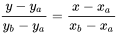
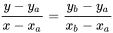
• Polynomial interpolation
• It is a generalization of linear interpolation.
• Polynomial interpolation can be used to estimate local maxima and minima that are outside the sample range.

• Spline interpolation.
• Like polynomial interpolation, spline interpolation produces less error than linear interpolation, while the interpolant is smoother and easier to evaluate than the high-degree polynomials used in polynomial interpolation.