Week 9 - FVM Literature Review

Finite difference method:

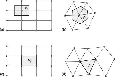
All grid points are in a straight line since the grid is linear and aligned in this way. The important thing is that the properties are thought to be concentrated in one location.

A body whose grid points are not properly aligned along the x and y directions cannot be directly modeled using FDM. These could happen as a result of intricate folds or cuts in the structure.

Finite element method:

Over an elemental area, the properties are applicable. properties that are thought to be concentrated in the area's center.

Finite volume method:

The approach is used across a volume so that the governing equation holds throughout the volume. It is also assumed that the characteristics are concentrated in the volume's geometric center.

A technique for expressing and analyzing partial differential equations as algebraic equations are known as the finite volume method (FVM). The divergence theorem is used in the finite volume technique to transform volume integrals in a partial differential equation including a divergence term into surface integrals. The surfaces of each finite volume are then used to assess these terms as fluxes. These approaches are conservative because the flux entering a particular volume is the same as the flux exiting the neighboring volume. The finite volume approach also has the benefit of being simply formulated to support unstructured meshes. Numerous software for computational fluid dynamics employs this technique. The little volume that surrounds each node point on a mesh is referred described as a "finite volume."

Steps:-

1. consider an equation in integral form.
2. Implement the Gauss Divergence Theorem.
3. We receive a discretized form called "Flux Terms," which can be solved using a computer.
4. Think about a heat conduction equation with heat production in a steady state:

`(delta )/(delta x) ( alpha . (delta T )/(delta x) ) + S = 0`

`alpha` is a thermal diffusivity term

`S` is a source term

`(delta T )/(delta x)` is temperature gradient along the x direction.

The "integral form of governing equation"—which should be equal to zero if a small control volume (dv) is taken into account, multiplied by the governing equation, and integrated over the full volume—should also be equal to zero.

Integrating the equation after multiplying it by "dv"

`int delta / (delta x) ( α . (delta T)/ (delta x) ) d v + int S d v = 0`

but `d v = A . d x`

`int delta / (delta x) ( α . (delta T)/ (delta x) ) A dx + int S d v = 0`

`underset(w)([ alpha A ( (delta T)/ (delta x )) ] ^e + overline(S)d v = 0`

`overline(S)` is an average value of source term (S)

`alphaunderset(e)() A ((delta T )/(delta x))underset(e)()-alphaunderset(w)() A ((delta T )/(delta x))underset(w)()+overlineSdv=0;`

If we assume α">αα as a constant and not a function of temperature,

`alphaA[(Tundersete() −Tundersetp())/(Δx)]−alphaA[(Tundersete() −Tundersetp())/(Δx)]+ overlineSdv=0`

`[Heatflux]underset(out)()−[Heatflux]underset(In)()+Source term=0`

Different schemes are used to solve the equation:

1. Gradient Scheme

The process of using temperature from a nearby point to estimate or numerically express the temperature gradient on the east face, as shown in the above diagram, is known as the gradient scheme.

2. Interpolation scheme

Evaluation of surface and volume integrals in the finite volume formulation occasionally calls for the values of the unknown variables to be located somewhere other than the computational nodes of the control volume. These values are acquired by the use of certain interpolation techniques.

Let's use the straightforward situation of stable one-dimensional convection and diffusion as an illustration.

`(d)/( d x) ( rho u phi) = (d)/( d x) ( Gamma (dphi)/(dx))`

`phi`solution variable

`rho`is the density

`u` is the velocity

`Gamma` is the diffusion coefficient.

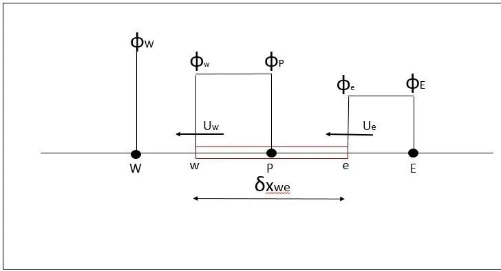
the control volume surrounding grid point P after integration of the governing differential equation produces:

`( rho u phi)undersete() - ( rho u phi)undersetw() = ( Gamma (dphi)/(dx))undersete() -( Gamma (dphi)/(dx))undersetw()`

The values of over-face “e” and “w” are necessary for evaluating the left-hand side of the above equation. These numbers are calculated using specific interpolation techniques.

The following are some interpolation techniques used in CFD:

1. upwind interpolation scheme
2. linear interpolation scheme
3. The QUICK technique (Quadratic Upwind Interpolation for Convective Kinematics)
4. Hybrid scheme
5. Total Variation Diminishing (TVD) scheme

Upwind interpolation scheme

The value of the solution variable at the face is estimated by its value at the upstream computational node under the Upwind interpolation technique, which considers the direction of fluid flow. For example, if the fluid is flowing eastward (see image),then

`phiundersete ()approx phiP`

Furthermore, if the fluid is flowing from east to west (see image), then

`phiundersete ()approx phiE`

Flux Limiters

As a result of shock, the variable gradients toggle when calculated, are not bounded to a specific value and jump. With a flux limiter, the gradient value can be limited, resulting in a stable solution.

While numerical approximation using higher-order spatial discretization schemes produces more accurate results, it also exhibits spurious oscillations near discontinuities like shocks. Despite being stable close to discontinuities, lower-order spatial discretization schemes dampen out distributions due to their dissipative nature. To capture discontinuities, high-resolution schemes must be extremely accurate and stable across domains.

Suppose represents flux at face e calculated using a high-resolution scheme, `Lundersete` represents flux at e calculated using a lower order scheme and `Hundersete` represents flux at e calculated using a higher order scheme. Then `psi(r)` represents the flux limiter function such that:

`F undersete() = L undersete() +phi ( r ) ( H undersete() − L undersete() )`

Flux limiter function depends upon the smoothness parameter r which is defined as:

`rundersetP() = (phip-phiW)/(phiE-phiP)`

It is mandated that the flux limiter function be greater than or equal to zero. The value is assumed to be 0 when it is close to discontinuities and 1 when it is far from them. In order to numerically represent flux, it, therefore, alternates between higher order and lower order schemes, maintaining the scheme's accuracy and stability throughout.

Because they both have the same mathematical form and both have the same effect of limiting the solution gradient near shocks or discontinuities, it should be noted that flux limiters are also known as slope limiters. In general, a limiter that acts on system fluxes is referred to as a flux limiter, and a limiter that acts on system states is referred to as a slope limiter (like pressure, velocity, etc.).

consider 1D- semi-discrete scheme

`(d u underseti())/ (d t) + 1 /(Δ x underseti())[ F ( u underset(i+1/(2))() ) − F ( u underset(i-1/(2))() ) ] = 0`

`F ( u underset(i+1/(2))() ) &F ( u underset(i-1/(2))() )` these are edge fluxes for the i^th cell

`F ( u underset(i+1/(2))() ) = underset(i+1/(2))(f ^(low)) − phi ( r i ) ( underset(i+1/(2))(f ^(low)) -underset(i+1/(2))(f ^(high)) )`

`F ( u underset(i-1/(2))() ) = underset(i-1/(2))(f ^(low)) − phi ( r i ) ( underset(i-1/(2))(f ^(low)) -underset(i-1/(2))(f ^(high)) )`

`f^(high)` low precision, high resolution flux

`f^(low)`high precision , low-resolution flux

`phi(r)` flux limiter function

`runderseti() = (u underseti()-u underset(i-1)())/(u underset(i+1)()-u underset(i)())`

`phige0` `r` represents the ratio of successive gradients on the solution mesh

this is the limiter function case

if limiter function`=0`, then there will be a low resolution and sharp gradient.

if limiter function `gt0`, then there will be a high resolution and +ve gradient.