Week 3.5 - Deriving 4th order approximation of a 2nd order derivative using Taylor Table method
Foruth order approrimmation of the second order derivation
A) Central difference
a b c d e
(i-2) (i-1) (i) (i+1) (i+2)
`(d^2u)/(dx^2)= af(i-2)+bf(i-1)+cf(i)+df(i+1)+ef(i+2)`
here we computing 4th order approximation at point (i) by central differance method, by taking two value on both side of point (i)
to calcuate the coefficients of variables a,b,c,d,e by using Taylor table
| f(i) | `Deltax` f'(i) |
`Deltax^2` f''(i) |
`Deltax^3` f'''(i) |
`Deltax^4` f''''(i) |
`Deltax^5` f'''''(i) |
`Deltax^6` f''''''(i) |
|
| af(i-2) | a | `-2a` | `(4a)/2` | `-(8a)/6` | `(16a)/24` | `(-32a)/120` | `(64a)/720` |
| bf(i-1) | b | -b | `b/2` | `-b/6` | `b/24` | `-b/120` | `b/720` |
| cf(i) | c | 0 | 0 | 0 | 0 | 0 | 0 |
| df(i+1) | d | d | `d/2` | `d/6` | `d/24` | `d/120` | `d/720` |
| ef(i+2) | e | `2e` | `(4e)/2` | `(8e)/16` | `(16e)/24` | `(32e)/120` | `(64e)/720` |
| 0 | 0 | 1 | 0 | 0 | ?? | ?? |
here we have five unknows variables a,b,c,d,e and 5 equations by solving this eqations we can get coefficients
`a+b+c+d+e=0`
`-2a-b+d+2e=0`
`(4a)/2-b/2+d/2+(4e)/2=1`
`(-8a)/6+b/6+d/6+(8e)/6=0`
`(16a)/24+b/24+d/24+(16e)/24=0`
by solving this equation by matix AX=B
a=-0.833333
b=1.33333
c=-2.50000
d=1.333333
e=0.833333
after puting this values in our Taylo series the final equation will be the
`(∂ ^2 u )/( ∂ x ^2 ) = ( a + b + c + d + e ) f ( i ) + ( − 2 a − b + 0 + d + 2 e ) f ′ ( i ) Δ x + ( 2 a + b/2 + 0 + d/2+ 2 e ) f ′ ' ( i ) Δ x^ 2 + ( − (8a)/6− b/6 + 0 + d/6 + (8e )/6 )f ′ ' ' ( i ) Δ x^ 3 + ( (16 a)/24 + b/24 + 0 + d/24+ (16e)/ 24 ) f ′ ' ' ' ( i ) Δ x ^4 + ( −( 32a)/120 -b/120 + 0 + d/120 + (32e)/120 ) f ′ ' ' ' ' ( i ) Δ x ^5 + ( (64a)/ 720 + b /720 + 0 + 1/720 + (64 e)/720 ) f ′ ' ' ' ' ' ( i ) Δ x ^6`
final equation will be
`(∂ ^2 u)/ ( ∂ x 2 ) = ( 2 ( − 0.083333 ) + 1.333333 2 + 1.333333 2 + 2 ( 0.083333 ) ) f ′ ' ( i ) + ( 64 240 ( − 0.083333 ) + 1.333333 240 + 1.333333 240 + 64 240 ( 0.083333 ) ) f ′ ' ' ' ' ' ( i ) Δ x 4`
form above Eq `Deltax^4` is truncation error. The order of the approximaton is define by the truncation error, Now we can say that our central differance scheme is 4th order.
B) Skewed right-sided difference
a b c d e g
(i) (i+1) (i+2) (i+3) (i+4) (i+5)
`(d^2u)/(dx^2)= af(2)+bf(i+1)+cf(i+2)+df(i+3)+ef(i+4)+gf(i+5)`
here we computing 4th order approximation at point (i) by Skewed right-sided difference method, by taking five value on right side of point (i)
to calcuate the coefficients of variables a,b,c,d,e by using Taylor table
| f(i) | `Deltax` f'(i) |
`Deltax^2` f''(i) |
`Deltax^3` f'''(i) |
`Deltax^4` f''''(i) |
`Deltax^5` f'''''(i) |
`Deltax^6` f''''''(i) |
|
| af(i) | a | 0 | 0 | 0 | 0 | 0 | 0 |
| bf(i+1) | b | b | `b/2` | `b/6` | `b/24` | `b/120` | `b/720` |
| cf(i+2) | c | 2c | `(4c)/2` | `(8c)/6` | `(16c)/24` | `(32c)/120` | `(64c)/720` |
| df(i+3) | d | 3d | `(3d)/2` | `(27d)/6` | `(81d)/24` | `(243d)/120` | `(729d)/720` |
| ef(i+4) | e | `4e` | `(16e)/2` | `(16e)/16` | `(256e)/24` | `(1024e)/120` | `(4096e)/720` |
| gf(i+5) | g | 5g | `(25g)/2` | `(125g)/6` | `(625g)/24` | `(3125g)/120` | `(15625g)/720` |
| 0 | 0 | 1 | 0 | 0 | 0 | ?? |
here we have five unknows variables a,b,c,d,e,g and 6 equations by solving this eqations we can get coefficients
`a+b+c+d+e=0`
`0+b+2c+3d+4e=0`
`0+b/2+2c+(9d)/2+8e=1`
`0+b/6+(8c)/6+(27d)/6+(64e)/6=0`
`0+b/24+(16c)/24+(81d)/24+(256e)/24=0`
`0+b/120+(32c)/120+(243d)/120+(1024e)/120+(3125g)120=0`
by solving this equation by matix AX=B
`a=3.7500`
`b=-12.8333`
`c=17.8333`
`d=-13.00000`
`e=5.08333`
`g=-0.833333`
after puting this values in our Taylo series the final equation will be the
`(d^2u)/(dx^2)= (af(i)+bf(i+1)+cf(i+2)+df(i+3)+ef(i+4)+g(i+5))/(Deltax^2)`
after putting coifficient values in the equatioin the final will be
`(∂ ^2 u)/( ∂ x^ 2) = ( 0+b/2 + (4 c)/2 + (9 d)/ 2 + (16e)/2+(25g)/2 ) f ′ ' ( i ) + ( b /720 + (64 c)/ 720 + (729 d )/720 + (4096 e)/ 720+(15625g)/720) f ′ ' ' ' ' ' ( i ) Δ x ^4`
form above Eq `Deltax^4` is truncation error. The order of the approximaton is define by the truncation error, Now we can say that our Skewed right-sided difference scheme is 4th order.
C)Skewed left-sided difference
a b c d e g
(i-5) (i-4) (i-3) (i-2) (i-1) (i)
`(d^2u)/(dx^2)= af(i-5)+bf(i-4)+cf(i-3)+df(i-2)+ef(i-1)+gf(i)`
here we computing 4th order approximation at point (i) by Skewed Lift-sided difference method, by taking five value on left side of point (i)
to calcuate the coefficients of variables a,b,c,d,e by using Taylor table
| f(i) | `Deltax` f'(i) |
`Deltax^2` f''(i) |
`Deltax^3` f'''(i) |
`Deltax^4` f''''(i) |
`Deltax^5` f'''''(i) |
`Deltax^6` f''''''(i) |
|
| af(1-5) | a | -5a |
`(25a)/2` |
`(-125a)/6` |
`(625a)/24` |
`(-3125a)/120` |
`(15625a)/720` |
| bf(i-4) | b |
`-4b`` |
`8b` | `-(64b)/6` | `(256b)/24` | `(-1024b)/120` | `(4096b)/720` |
| cf(i-3) | c | -3c | `(9c)/2` | `(-27c)/6` | `(81c)/24` |
`(-243c)/120` |
`(729c)/720` |
| df(i-2) | d | -d | -2d | `(-8d)/6` | `(16d)/24` | `(-32d)/120` | `(64d)/720` |
| ef(i-1) | e | -e | `e/2` | `-e/6` | `e/24` | `-e/120` | `e/720` |
| gf(i) | g | 0 | 0 | 0 | 0 | 0 | 0 |
| 0 | 0 | 1 | 0 | 0 | 0 | ?? |
here we have five unknows variables a,b,c,d,e,g and 5 equations by solving this eqations we can get coefficients
`a+b+c+d+e=0`
`-4a-3b-2c-d+0=0`
`8a+(9b)/2+2d+(e)/2+0=1`
`-(64a)/6-(27b)/6+(8c)/6-(d)/6+0=0`
`(256a)/24+(81b)/24+(32c)/120-(d)/120+0=0`
`(-3125a)/120-(1024b)/120-(243c)/120-(32d)/120-e/120+0=0`
by solving this equation by matix AX=B
`a=-0.8333`
`b=-5.0833`
`c=-13.000`
`d=17.8333`
`e=-12.8333`
`g=3.75000`
after puting this values in our Taylo series the final equation will be the
`(d^2u)/(dx^2)= (af(i-5)+bf(i-4)+cf(i-3)+df(i-2)+ef(i-1)+gf(i))/(Deltax^2)`
after putting coifficient values in the equatioin the final will be
`(∂ ^2 u)/( ∂ x^ 2) = ( (25a)/2+ 8b + (9c)/2 + 2d+e/2+0 ) f ′ ' ( i ) + ((15625a)/720+(4096a) /720 + (729b)/ 720 + (64c )/720 + d/ 720+e/720) f ′ ' ' ' ' ' ( i ) Δ x ^4`
form above Eq `Deltax^4` is truncation error. The order of the approximaton is define by the truncation error, Now we can say that our Skewed left-sided difference scheme is 4th order.
Program for the Foruth order Approximation of the second order derivation
We wrtie code to develep the function for central differance,skewed right and left side for a particular point(x,dx) dx repersent the each node range.
The function returns the foruth order approximation and we find out the error differance b/w the analytical sol and central sekwed right and left side for range the of dx
Code for the Central differance method
%coding for central differance method

function out1= central_differance(x,dx)

% fuction f(x) = exp(x)*cos(x)
 % Analytical sol of second order f''(x)=-2*exp(x)*sin(x)

       Analytical_sol= -2*exp(x)*sin(x);
       a1 =[1 1 1 1 1; -2 -1 0 1 2; 2 1/2 0 1/2 2; -8/6 -1/6 0 1/6 8/6; 16/24 1/24 0 1/24 16/24];
       b1=[0; 0; 1; 0; 0];
       coeff= linsolve(a1,b1);

       % values of coifficients of variables form taylor table
       a=coeff(1);
       b=coeff(2);
       c=coeff(3);
       d=coeff(4);
       e=coeff(5);

       % computing the 4th order approximation by central differance method
       % central differanceing =
       % (af(x-2dx)+bf(x-dx)+cf(x)+df(x+dx)+ef(x+2dx))/(2^dx)

       p= (exp(x-2*dx)*cos(x-2*dx));
      q = (exp(x-dx)*cos(x-dx));
       r=  (exp(x)*cos(x));
       s=  (exp(x+dx)*cos(x+dx));
       t=  (exp(x+2*dx)*cos(x+2*dx));

       central_differance = ((a*p) + (b*q) + (c*r) + (d*s) + (e*t))/(dx^2);


       % computing error b/w analytical sol and central differance

       out1= abs(central_differance-Analytical_sol);

       end
Code for Skewed Right side method
%coding for skewed right side differance

function out2= skewed_right_sided_difference (x,dx)

% fuction f(x) = exp(x)*cos(x)
 % Analytical sol of second order f''(x)=-2*exp(x)*sin(x)

       Analytical_sol= -2*exp(x)*sin(x);
       c1 = [1 1 1 1 1 1; 0 1 2 3 4 5; 0 1/2 2 9/2 8 25/2; 0 1/6 8/6 27/6 64/6 125/6; 0 1/24 16/24 81/24 256/24 625/24; 0 1/120 32/120 243/120 1024/120 3125/120];
       d1 = [0; 0; 1; 0; 0; 0];
       coeff= linsolve(c1,d1);

       % values of coifficients of variables form taylor table
       a=coeff(1);
       b=coeff(2);
       c=coeff(3);
       d=coeff(4);
       e=coeff(5);
       g=coeff(6);


       % computing the 4th order approximation by skewed right side differance
       % skewed right side differance =
       % (af(x)+bf(x+dx)+cf(x+2*dx)+df(x+3*dx)+ef(x+4*dx)+gf(x+5*dx)/(2^dx)

       p= (exp(x)*cos(x));
      q = (exp(x+dx)*cos(x+dx));
       r=  (exp(x+2*dx)*cos(x+2*dx));
       s= (exp(x+3*dx)*cos(x+3*dx));
       t=  (exp(x+4*dx)*cos(x+4*dx));
       v = (exp(x+5*dx)*cos(x+5*dx));

       right_side_differance = ((a*p) + (b*q) + (c*r) + (d*s) + (e*t) + (g*v))/(dx^2);


       % computing error b/w analytical sol and skewed right side differance

       out2= abs(right_side_differance -Analytical_sol);

       end
Code for Skewed left side method
%coding for skewed left side differance

function out3 = skewed_left_sided_difference (x,dx)

% fuction f(x) = exp(x)*cos(x)
 % Analytical sol of second order f''(x)=-2*exp(x)*sin(x)

       Analytical_sol= -2*exp(x)*sin(x);
       l1 = [1 1 1 1 1 1; -5 -4 -3 -2 -1 0; 25/2 16/2 9/2 4/2 1/2 0; -125/6 -64/6 -27/6 -8/6 -1/6 0; 625/24 256/24 81/24 16/24 1/24 0; -3125/120 -1024/120 -243/120 -32/120 -1/120 0];
       m1 = [0; 0; 1; 0; 0; 0];
       coeff= linsolve(l1,m1);

       % values of coifficients of variables form taylor table
       a=coeff(1);
       b=coeff(2);
       c=coeff(3);
       d=coeff(4);
       e=coeff(5);
       g=coeff(6);


       % computing the 4th order approximation by skewed right side differance
       % skewed right side differance =
       % (af(x)+bf(x+dx)+cf(x+2*dx)+df(x+3*dx)+ef(x+4*dx)+gf(x+5*dx)/(2^dx)

       p= (exp(x-5*dx)*cos(x-5*dx));
      q = (exp(x-4*dx)*cos(x-4*dx));
       r=  (exp(x-3*dx)*cos(x-3*dx));
       s= (exp(x-2*dx)*cos(x-2*dx));
       t=  (exp(x-dx)*cos(x-dx));
       v =  (exp(x)*cos(x));

       left_side_differance = ((a*p) + (b*q) + (c*r) + (d*s) + (e*t) + (g*v))/(dx^2);


       % computing error b/w analytical sol and skewed left side differance

       out3= abs(left_side_differance - Analytical_sol);

       end
Code for the Main Function
In Main function we create array for the range of dx
we use for loop over dx range and call the fuction central differance, sekwed right and left side
now we get the error over the range of dx and pot graph for the error vx dx for all 3 methods
clear all
close all
clc
 x=pi/3;
 dx=linspace(pi/40,pi/4000,100);

 for i=1:length(dx)

     error_central(i)= central_differance(x,dx(i));
     error_right(i) = skewed_right_sided_difference(x,dx(i));
     error_left(i) =skewed_left_sided_difference(x,dx(i));
 end
%plotting graphs for dx vs errors for central, skewed right-sided, & skewed left-sided approximations

figure(1)
plot(dx,error_central,'linewidth',2)
hold on
grid on
plot(dx,error_right,'r','linewidth',2)
hold on
plot(dx,error_left,'g','linewidth',2)
xlabel('dx')
ylabel('error')
legend('Central Difference Error','Skewed Right-Sided Error','Skewed Left-Sided Error')

figure(2)
loglog(dx,error_central,'linewidth',2)
hold on
grid on
loglog(dx,error_right,'r','linewidth',2)
hold on
loglog(dx,error_left,'g','linewidth',2)
xlabel('dx')
ylabel('error')
legend('Central Difference Error','Skewed Right-Sided Error','Skewed Left-Sided Error')
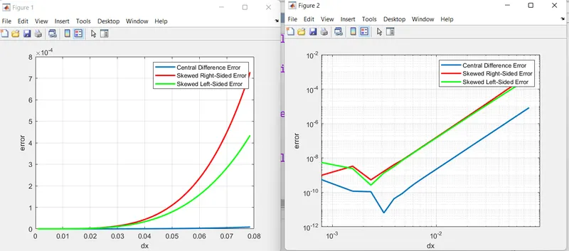
Results
we can observe form the graph, the central differance method has high accuracy solutions and less error when we compare with remaining two methods
but we cant use Central differance at some situation i.e., we cant evaluate solution at boundary or corner node, then we can use skewed methods bcoz its take data form one side to evaluate numerical approximation.