Week 9 - FVM Literature Review

Finite Volume Method:-

Finite Volume refers to the small volume sourrounding each node point on a mesh. The Finite volume method (FVM) is a method for representing and to evaluating partial differential equations in the form of algebraic equations.

In finite volume method, volume integrals in a partial differential equation that contain a divergence term are converted to surface integrals(Based on using the divergence theorem). These terms are then evaluated as fluxes at the surfaces of each finite volume, the flux that entering a given volume is identical to that leaving the adjacent volumes(these methods are conservative).

Another one such advantage of the finite volume method is that it is easily formulated to allow for unstructured meshes. The above method is used in many computational fluid dynamic packages.

In finite volume method, first the flow geometry is defined. Then the flow domain is decomposed into a computational mesh or grid(a set of non-overlapping control volumes or cells).Such that the integral equations are to be discretized, ie , approximated in terms of values at a set of nodes, then the discretized equations are solved numerically.

Differences between FDM and FVM:-

• Finite difference Method (FDM) are introduced by Euler in 18th centuary.
• The finite difference method (FDM) is an approximate method for solving partial differential equations. It has been used to solve a wide range of problems. These include linear and non-linear, time independent and dependent problems.
• This method can be applied to problems with different boundary shapes, different kinds of boundary conditions, and for a region containing a number of different materials.
• The application of FDM is not difficult as it involves only simple arithmetic in the derivation of the discretization equations and in writing the corresponding programs.
• During 1950–1970 FDM was the most important numerical method used to solve practical problems.
• It is difficult to satisfy conservation and to apply for irregular geometries
• Finte Volume Metod (FVM)-The finite volume method (FVM) is a discretization technique for partial differential  equations, especially those that arise from physical conservation laws.
• FVM can accommodate any type of grid, so it is suitable for complex geometries.
• FVM is similar to FDM but the method (FVM) integrates the differential equation over a control volume and discretizing the domain.
• It tends to be biased toward edges and one-dimensional physics.
• The disadvantage of FVMs compared with FD schemes is that methods of order higher than second are more difficult to develop in 3D.

Interpolation schemes in Finite Volume Method(FVM)

1. Upwind Interpolation Scheme(UDS)
2. Central Differencing Approximations(CDS)
3. Quadratic Upwind Differencing Scheme(QUICK)
4. Hybrid interpolation Scheme(CDS & UDS)
5. Total Variation Diminishing Scheme(TVD)

Upwind Interpolation Scheme(UDS)

• In this scheme we use the node in the upwind or upstream of the given node. it is generally used for convection dominated problems. The upwind interpolation for approximating the value of a variable 'f 'at the east face of a control volume is given by

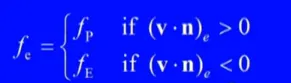
• UDS is equivalent to using a backward or forward finite difference approximation(depending on the flow direction)

Upwind interpolation is the only approximation that satisfies boundedness criterion unconditionally. unconditionally in the sense that  irrespective of what the velocity values are and irrespectiive of what is the grid spacing the solution will always remain bounded that is this use of upwind interpolation,will never yield oscillatoryy solutions.

• Disadvantages of UDS is numerically diffusive.
• Numerical diffusion is magnified in multidimensional problems if flow is oblique to the grid.
• Peak or rapid variations in the variables will be smeared out. 
• Only first order accurae. Hence, very fine grids are required to obtain accurate solutions.

Linear Interpolation(CDS)

• Approximates the values of the variable at CV face centre by linear interpolation of the values at two nearest nodes.
• It is equivalent to the central differencing formula for the first order derivative and hence this termed as the Central Differencing Scheme.
• CDS is second order accurate on uniform grids, but formally of first order on a non uniform grid.
• Most widely used scheme as it results in simple approximations for evaluation of gradients required for the evaluation of diffusive fluxes.
• It may produce oscillatory solution.

Quadratic Upwind Differencing Scheme(QUICK)

• Approximate the value of the variable at control voume face centre by quadratic interpolation of the values at three nearest computational nodes( One downstream node D and two upstream node U, UU).
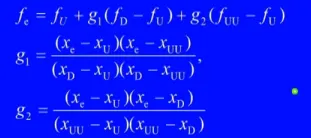
• Leonard (1979) named this scheme as QUICK(Quadric upwind interpolation for convective kinematics)
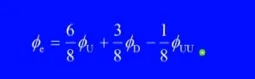
• It is third order accurate but is prone to oscillations and is derived from polynomial fittings. The interpolation on a uniform cartesian grid is given by
• 

Hybrid interpolation Scheme(CDS & UDS)

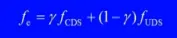
• Hybrid Inerpolation scheme:Blend of CDS and UDS scheme based on local peclet number.

        

Total Variation Diminishing Scheme(TVD)

     

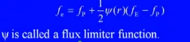
Flux Limiter

They are used in high resolution schemes, to avoid the false oscillations that would otherwise occur with high order spatial discretization schemes due to shocks,discontinuities or sharp changes in th solution domain.Use of flux limiters, together with an appropriate high resolution scheme, make the solutions total variation diminishing (TVD). The main idea behind the construction of flux limiter schemes is to limit the spatial derivatives to realistic values.The main purpose of flux limiter is to keep the values bounded at the cell faces. Flux limiter dont let the solution value to overshoot.

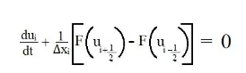
Consider a 1D semi Discrete scheme

w

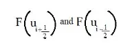
where the above represents the edge fluxes for the 'i' th cell can be represented by low and high resolution schemes then the flux limiter can switch between these scheme depending upon the gradients close to the particular cell.

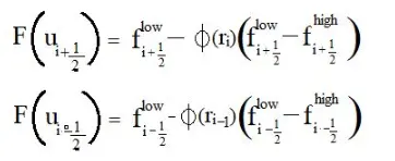
f^low  = low Resolution flux.

f^high = high Resolution flux.

Φ(r) = Flux limiter function.

and 'r' represents the ratio of sucessive gradients on the solution mesh, ie;

r_i = (u_i-u_i-1 )/(u_i+1-u_i)