Week 3.5 - Deriving 4th order approximation of a 2nd order derivative using Taylor Table method
objective:-
To derive the fourth order approximations of a second order derivative using , skewed right sided difference, skewed left sided difference and central differencing scheme with the help of a taylor table method and to compare the analytical derivative with obtained values for the given function.
Derive the fourth order approximations of the second derivative.
1) Skewed right sided difference.
Number of nodes required for fourth order approximation of a second order derivative can be given by the equation,
N= P+Q where
N - No of nodes.
P - Order of approximations.
Q - Order of derivative.
Here we are using 6 nodes inorder to find the second order derivative with the fourth order of approximation.
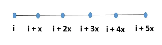
Formulation for the taylor table method of Right skewed scheme.

Using taylor series to find the values of discrete points with respect to point i.
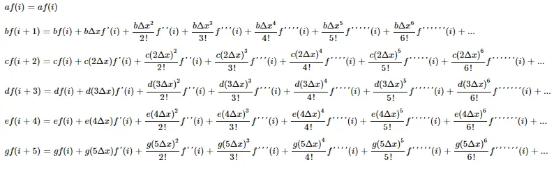
Adding LHS nad RHS from the above equation.
While looking into the above equations, we wnt only the coefficients of Δx^2 f''(i) and assume the coefficient to be one and for the remaining terms, assume the coefficient to be zero.
ie;
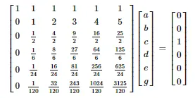
a + b + c + d + e + g =0
b + 2c + 3d + 4e + 5g = 0
b/2 + 4c/2 + 9d/2 + 16e/2 +25g/2 = 1
b/6 + 8c/6 + 27d/6 + 64e/2 + 125g/6 = 0
b/24 + 16c/24 + 81d/24 + 256e/24 + 625g/24 = 0
b/120 + 32c/120 + 243d/120 + 1024e/120 + 3125g/120 = 0
Fourth order right skewed scheme.
|
Taylor Table |
|||||||
|
Function |
Taylor series expansion |
||||||
|
f(i) |
Δf’(i) |
Δx2f’’(i) |
Δx3f’’’(i) |
Δx4f’’’’(i) |
Δx 5f’’’’’(i) |
Δx6 f’’’’’’(i) |
|
|
af(i) |
a |
0 |
0 |
0 |
0 |
0 |
0 |
|
bf(i+1) |
b |
b |
b/2 |
b/6 |
b/24 |
b/120 |
b/720 |
|
cf(i+2) |
c |
2c |
4c/2 |
8c/6 |
16c/24 |
32c/120 |
64c/720 |
|
df(i+3) |
d |
3d |
9d/2 |
27d/6 |
81d/24 |
243d/120 |
729d/720 |
|
ef(i+4) |
e |
4e |
16e/2 |
64e/6 |
256e/24 |
1024e/120 |
4096e/720 |
|
gf(i+5) |
g |
5g |
25g/2 |
125g/6 |
625g/24 |
3125g/120 |
15625g/720 |
|
Sum of coefficients |
0 |
0 |
1 |
0 |
0 |
0 |
? |
Writing the above coefficients in the form of a matrix;
2) Skewed left sided difference.
Number of nodes required for fourth order approximation of a second order derivative can be given by the equation,
N= P+Q where
N - No of nodes.
P - Order of approximations.
Q - Order of derivative.
Here we are using 6 nodes inorder to find the second order derivative with the fourth order of approximation.
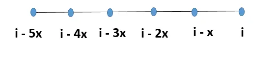
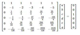
Formulation for the taylor table method of left skewed scheme.

Fourth order left skewed scheme.
|
Taylor Table |
|||||||
|
Function |
Taylor series expansion |
||||||
|
f(i) |
Δf’(i) |
Δx2f’’(i) |
Δx3f’’’(i) |
Δx4f’’’’(i) |
Δx 5f’’’’’(i) |
Δx6 f’’’’’’(i) |
|
|
af(i) |
a |
0 |
0 |
0 |
0 |
0 |
0 |
|
bf(i-1) |
b |
-b |
b/2 |
-b/6 |
b/24 |
-b/120 |
b/720 |
|
cf(i-2) |
c |
-2c |
4c/2 |
-8c/6 |
16c/24 |
-32c/120 |
64c/720 |
|
df(i-3) |
d |
-3d |
9d/2 |
-27d/6 |
81d/24 |
-243d/120 |
729d/720 |
|
ef(i-4) |
e |
-4e |
16e/2 |
-64e/6 |
256e/24 |
-1024e/120 |
4096e/720 |
|
gf(i-5) |
g |
-5g |
25g/2 |
-125g/6 |
625g/24 |
-3125g/120 |
15625g/720 |
|
Sum of coefficients |
0 |
0 |
1 |
0 |
0 |
0 |
? |
Writing the above coefficients in the form of a matrix;
2) Central difference.
Number of nodes required for fourth order approximation of a second order derivative can be given by the equation,
N= P+Q-1 where
N - No of nodes.
P - Order of approximations.
Q - Order of derivative.
Here we are using 5 nodes inorder to find the second order derivative with the fourth order of approximation.
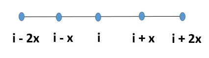
Formulation for the taylor table method of Central difference scheme.

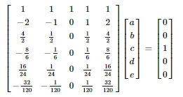
Central difference scheme
|
Taylor Table |
|||||||
|
Function |
Taylor series expansion |
||||||
|
f(i) |
Δxf’(i) |
Δx2f’’(i) |
Δx3f’’’(i) |
Δx4f’’’’(i) |
Δx 5f’’’’’(i) |
Δx6 f’’’’’’(i) |
|
|
af(i-2) |
a |
-2a |
4a/2 |
-8a/6 |
16a/24 |
-32a/120 |
64a/720 |
|
bf(i-1) |
b |
-b |
b/2 |
-b/6 |
b/24 |
-b/120 |
b/720 |
|
cf(i) |
c |
0 |
0 |
0 |
0 |
0 |
0 |
|
df(i+1) |
d |
d |
d/2 |
d/6 |
d/24 |
-c/120 |
d/720 |
|
ef(i+2) |
e |
2e |
4e/2 |
-8e/6 |
16e/24 |
32e/120 |
64e/720 |
|
Sum of coefficients |
0 |
0 |
1 |
0 |
0 |
? |
? |
Writing the above coefficients in the form of matrix, we get,
Matlab program
% Initialization
clear
close all
clc

% Values of x and dx

x = pi/3;
dx= linspace(pi/4,pi/400,200);

% Given Function

% function = exp(x)*cos(x);
% Analytical value = -2*exp(x)*sin(x);

Analytical_derivative = -2*exp(x)*sin(x);

% Left side skewed

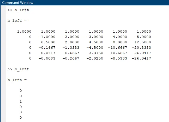
a_left = [1 1 1 1 1 1 ; 0 -1 -2 -3 -4 -5 ; 0 1/2 4/2 9/2 16/2 25/2 ; 0 -1/6 -8/6 -27/6 -64/6 -125/6 ; 0 1/24 16/24 81/24 256/24 625/24 ; 0 -1/120 -32/120 -243/120 -1024/120 -3125/120];
b_left = [0; 0; 1; 0; 0; 0;];
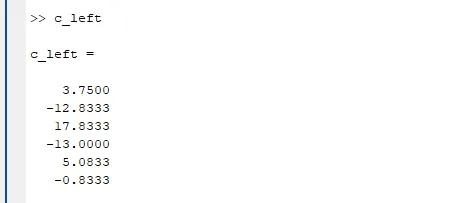
c_left = inv(a_left)*b_left;

skewed_left = (c_left(1).*exp(x).*cos(x) + c_left(2).*exp(x-dx).*cos(x-dx) + c_left(3).*exp(x-2*dx).*cos(x-2*dx) + c_left(4).*exp(x-3*dx).*cos(x-3*dx) + c_left(5).*exp(x-4*dx).*cos(x-4*dx)+ c_left(6).*exp(x-5*dx).*cos(x-5*dx))./(dx.^2);

% Error calculation for left side skewed
error_left = abs(skewed_left - Analytical_derivative);


% Right side skewed

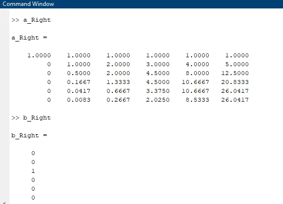
a_Right = [1 1 1 1 1 1 ; 0 1 2 3 4 5 ; 0 1/2 4/2 9/2 16/2 25/2 ; 0 1/6 8/6 27/6 64/6 125/6 ; 0 1/24 16/24 81/24 256/24 625/24 ; 0 1/120 32/120 243/120 1024/120 3125/120];
b_Right = [0; 0; 1; 0; 0; 0;];
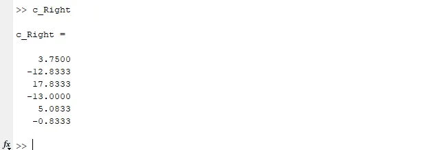
c_Right = inv(a_Right)*b_Right;

skewed_Right = (c_Right(1).*exp(x).*cos(x) + c_Right(2).*exp(x+dx).*cos(x+dx) + c_Right(3).*exp(x+2*dx).*cos(x+2*dx) + c_Right(4).*exp(x+3*dx).*cos(x+3*dx) + c_Right(5).*exp(x+4*dx).*cos(x+4*dx)+ c_Right(6).*exp(x+5*dx).*cos(x+5*dx))./(dx.^2);

% Error calculation for Right side skewed
error_Right = abs(skewed_Right - Analytical_derivative);

% Central differencing
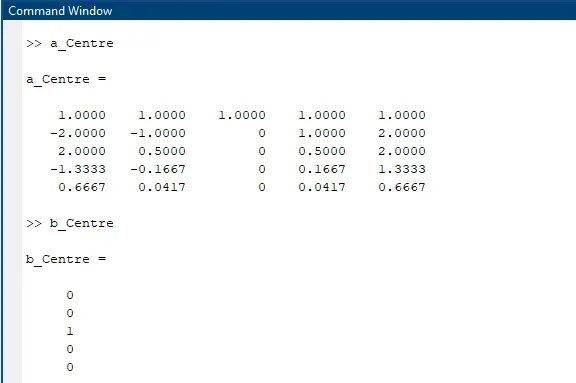
a_Centre = [1 1 1 1 1 ; -2 -1 0 1 2 ; 4/2 1/2 0 1/2 4/2 ; -8/6 -1/6 0 1/6 8/6 ; 16/24 1/24 0 1/24 16/24];
b_Centre = [0; 0; 1; 0; 0;];
c_Centre = inv(a_Centre)*b_Centre;

Centre_difference = (c_Centre(1).*exp(x-2*dx).*cos(x-2*dx) + c_Centre(2).*exp(x-dx).*cos(x-dx) + c_Centre(3).*exp(x).*cos(x) + c_Centre(4).*exp(x+dx).*cos(x+dx) + c_Centre(5).*exp(x+2*dx).*cos(x+2*dx))./((dx).^2);

% Error calculation for Central differencing.
error_Centre = abs(Centre_difference - Analytical_derivative);

% Plotting

loglog(dx,error_left,'LineWidth',2,'color','r');
hold on
loglog(dx,error_Right,'LineWidth',2,'color','g');
loglog(dx,error_Centre,'LineWidth',2,'color','b');
grid on
xlabel('dx');
ylabel('Error');
legend('Skewed left-side','Skewed Right-side','Central Differencing');
Coefficients for Skewed right side scheme,
Coefficients for Skewed Left side scheme,
Coefficients for Central difference,
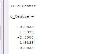
For calculating error all the three differencing schemes following expressions are used;
error_left = abs(skewed_left - Analytical_derivative).
error_Right = abs(skewed_Right - Analytical_derivative).
error_Centre = abs(Centre_difference - Analytical_derivative).
PLOT
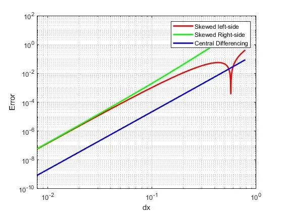
From the above graph we can conclude that the error of the central difference scheme is much lesser than the right and left skewed mehods. Here the right and left skewed difference methods almost give the same results in terms of error for a small value of time step.
Benefits of skewed scheme over central differencing scheme;
In order to apply the approximation scheme at boundaries, only skewed schemes are applicable. Due to unavailability if grid points on one sides of the boundary, central differencing scheme can't be applied because, central difference scheme requires number of grid points on both sides of the reference points, depending on the order of the approximation scheme and order of derivative to be evaluated.
So predicting the data from the central differencing is not possible, hence a skewed scheme plays a very important role in such cases.