Week 9 - FVM Literature Review
Finite Volume Method(FVM):
The Finite Volume Method (FVM) is the name given to the technique by which the integral formulation of the conservation laws is discretized directly in the physical space. It is the most widely applied method today in CFD. The reason behind the appeal to the FVM lies in its generality, its conceptual simplicity, and its ease of implementation for arbitrary grids structured as well as unstructured. FVM is based on cell-averaged values, which appear as the most fundamental quantity in CFD. This distinguishes the FVM from the finite difference and finite element methods, where the main numerical quantities are the local function values at the mesh points. Once a grid has been generated, the FVM consists in associating a local finite volume, also called control volume, to each mesh point and applying the integral conservation law to this local volume. This is the first major distinction from the finite difference approach, where the discretized space is considered as a set of points, while in the FVM the discretized space is formed by a set of small cells, one cell being associated to one mesh point.
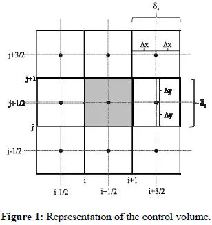
The application of FVM consists basically of subdividing the problem domain into elementary control volumes, as illustrated in Figure 1, and integrating each of those partial differential equations in these volumes, resulting in a nonlinear algebraic system, composed, in the two-dimensional case, by the equations presented below:
The strength of the FVM is its direct connection to the physical flow properties. Indeed, the basis of the method relies on the direct discretization of the integral form of the conservation law. This distinguishes the FVM significantly from the finite difference method.
The integral form is the most general expression of a conservation law, as it does not require the fluxes to be continuous (property which is not satisfied for instance along shock waves or along free surfaces). This is why we can state that the FVM is close to the physics of the flow system.
The FVM requires setting up the following steps:
- Subdivide the mesh, obtained from the space discretization, into finite (small)
volumes, one control volume being associated to each mesh point.
- Apply the integral conservation law to each of these finite volumes.
Major differences between FDM & FVM:
A finite difference method (FDM) discretization is based upon the differential form of the PDE to be solved. Each derivative is replaced with an approximate difference formula (that can generally be derived from a Taylor series expansion). The computational domain is usually divided into hexahedral cells (the grid), and the solution will be obtained at each nodal point. The FDM is easiest to understand when the physical grid is Cartesian, but through the use of curvilinear transforms the method can be extended to domains that are not easily represented by brick-shaped elements. The discretization results in a system of equations of the variable at nodal points, and once a solution is found, then we have a discrete representation of the solution.
A finite volume method (FVM) discretization is based upon an integral form of the PDE to be solved (e.g. conservation of mass, momentum, or energy). The PDE is written in a form that can be solved for a given finite volume (or cell). The computational domain is discretized into finite volumes and then for every volume, the governing equations are solved. The resulting system of equations usually involves fluxes of the conserved variable, and thus the calculation of fluxes is very important in FVM. The basic advantage of this method over FDM is it does not require the use of structured grids, and the effort to convert the given mesh into a structured numerical grid internally is completely avoided. As with FDM, the resulting approximate solution is discrete, but the variables are typically placed at cell centers rather than at nodal points. This is not always true, as there are also face-centered finite volume methods. In any case, the values of field variables at non-storage locations (e.g. vertices) are obtained using interpolation.
Need for interpolation schemes and flux limiters in FVM.
The use of interpolation schemes to approximate the property values located at the boundaries of the control volumes is necessary when FVM is applied, using as interpolation nodes the correspondent properties located at the center of the adjacent control volumes. Low-order schemes are commonly considered, due to their numerical stability and readiness of implementation. However, these schemes demand the use of a high degree of refinement of the meshes due to their lack of accuracy. Low-order interpolation schemes can lead to inaccurate results provoked by numerical diffusion effects. Alternatively, high-order interpolation schemes produce more accurate solutions with low computational costs. However, to maintain the global order of the approximation, it is important that all approximation formulas for the advective, diffusive, and nonlinear terms have the same order of accuracy.
Flux limiters
Most of us might have seen the behavior of numerical schemes in order to capture shocks and discontinuity that arises in hyperbolic equations. Physically, these equations model the convective fluid flow. It has been observed that low-order schemes are usually stable but quite dissipative in nature around the points of discontinuity/shocks. On the other hand higher-order, numerical schemes are unstable in nature and show oscillations in the vicinity of discontinuity. One can have a better understanding of such behavior by analyzing the modified equation of these schemes.
Now as said above one can not have high order accuracy without oscillations. The objective is to have highly accurate and stable oscillation-free schemes. This kind of scheme is known as a high-resolution scheme. Here we talk only about using the flux limiters function to construct high-resolution schemes. The idea is to tune the numerical flux of high order and low order scheme using the flux limiter function in such a way that the resulting scheme gives a high order accuracy in the smooth region of flow and sticks with the first order of accuracy in the vicinity of socks/discontinuities as follows:
Define the numerical flux fuction of high resolution conservative scheme as
F_(j+1/2) = L_(j+1/2) + phi (H_(j+1/2) - L_(j+1/2))
where L, H are the numerical flux of conservative low order and high order schemes respectively. And is a function of smoothness parameter usually defined as
theta_j = frac(U_j-U_(j-1))(U_(j+1) -U_j
What remains next is to define the limiter function () in such a way that it satisfies at least the following properties:
remains positive
Satisfies (1) = 1
passes through a particular region known as the TVD region associated with the underlying scheme in order to guarantee the stability of the scheme.
1D linear heat conduction equation as an example.
Let us consider a one-dimensional steady-state heat conduction equation and discretize it using the finite volume method.
frac(delta)(delta x)(frac(alpha delta T)(delta x)) + S = 0 ………………….(1)
Where S is the source term responsible for heat generation
Consider a grid as shown in the following figure:
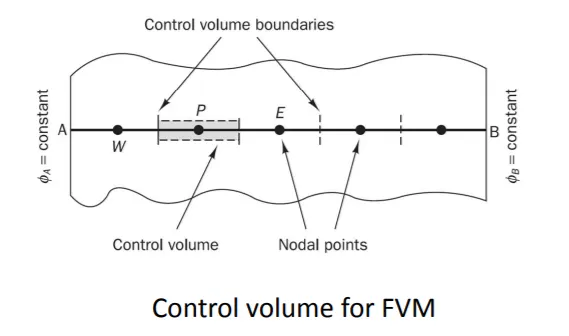
The solid dots are centers of a control volume so we are having an entire volume in between A and B. And inside these volumes equation (1) needs to be solved for its integral form.
Now consider a single volume P and its neighboring volumes W and E. The centers of the volumes are the solid nodes where the average quantities inside that volume are stored. Let w and e are phases that connect WP and PE respectively.
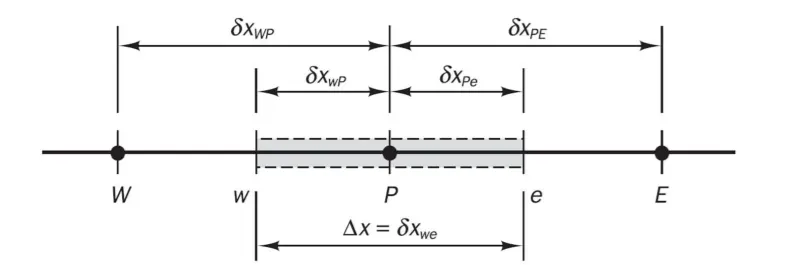
The integral form of equ (1) for a small value dV at any point over the volume will be-
int_w^e (frac(delta)(delta x)(alpha frac(delta T)(delta x) + S) dV = 0
int_w^e frac(delta)(delta x)(alpha frac(delta T)(delta x)) dV + int_w^e SdV = 0
int_w^e frac(delta)(delta x)(alpha frac(delta T)(delta x)) Adx + int_w^e SdV = 0
[(alpha A frac(delta T)(delta x))]_w ^e + bar S dV = 0
(alpha_e A frac(delta T)(delta x_e) - alpha_w A frac(delta T)(delta x_w)) + bar S dV = 0
alpha_e A [frac(T_E - T_P)(Delta x_e)] - alpha_w A [frac(T_P - T_W)(Delta x_w)] + bar S dV = 0 ………..(2)
The above equation is a conservation equation in Finite Volume Method form.
alpha_e A [frac(T_E - T_P)(Delta x_e)] and alpha_w A [frac(T_P - T_W)(Delta x_w)] terms represents the surface flux through the west and east interfaces of the control volume.
Interpretation:
The flux is being conserved inside the control volume. The flux entering the control volume through the west interface is equal to the sum of the flux leaving the control volume through the east interface and the heat generated within that control volume.