Week 5.1 - Mid term project - Solving the steady and unsteady 2D heat conduction problem

Theory:

Heat transfer has direction as well as magnitude. The rate of heat conduction in a specified direction is proportional to the temperature gradient, which is the rate of change in temperature with distance in that direction. Heat conduction in a medium, in general, is three-dimensional and time-dependent, and the temperature in a medium varies with a position as well as time, that

is, T T(x, y, z, t). Heat conduction in a medium is said to be steady when the temperature does not vary with time, and unsteady or transient when it does. Heat conduction in a medium is said to be one-dimensional when conduction is significant in one dimension only and negligible in the other two primary dimensions, two-dimensional when conduction in the third dimension is negligible, and three-dimensional when conduction in all dimensions is significant.

Steady State versus Transient State Heat Transfer:

Heat transfer problems are often classified as being steady (also called steady-state) or transient (also called unsteady). The term steady implies no change with time at any point within the medium, while transient implies variation with time or time dependence.

The temperature in a medium, in some cases, varies mainly in two primary directions, and the variation of temperature in the third direction (and thus heat transfer in that direction) is negligible. A heat transfer problem in that case is said to be two-dimensional. For example, the steady temperature distribution in a long bar of the rectangular cross-section can be expressed as T(x, y) if the temperature variation in the z-direction (along the bar) is negligible and there is no change with time.

Steady-state 2D heat conduction equation:

frac(d^2T)(dx^2)+frac(d^2T)(dy^2) = 0

Unsteady-state 2D heat conduction equation:

frac(delT)(delt) = alpha (frac(del^2T)(delx^2)+frac(del^2T)(dely^2))

Where, alpha = thermal diffusivity

Methods:

Numerical solution schemes are often referred to as being explicit or implicit. When a direct computation of the dependent variables can be made in terms of known quantities, the computation is said to be explicit. When the dependent variables are defined by coupled sets of equations, and either a matrix or iterative technique is needed to obtain the solution, the numerical method is said to be implicit.

In computational fluid dynamics, the governing equations are nonlinear, and the number of unknown variables is typically very large. Under these conditions implicitly formulated equations are almost always solved using iterative techniques.

Iterations are used to advance a solution through a sequence of steps from a starting state to a final, converged state. This is true whether the solution sought is either one step in a transient problem or a final steady-state result. In either case, the iteration steps resemble a time-like process.

Iterative methods:

In computational mathematics, an iterative method is a mathematical procedure that uses an initial value to generate a sequence of improving approximate solutions for a class of problems, in which the n-th approximation is derived from the previous ones. A specific implementation of an iterative method, including the termination criteria, is an algorithm of the iterative method. An iterative method is called convergent if the corresponding sequence converges for given initial approximations. The implicit scheme includes three iterative methods viz. Jacobi, Gauss-seidel, and Successive over-relaxation methods.

1. Jacobi method:

The Jacobi method is an iterative algorithm for determining the solutions of a strictly diagonally dominant system of linear equations.

1. Gauss-Seidel method:

the Gauss-Seidel method is an iterative method used to solve a system of linear equations. It is similar to the Jacobi method. Though it can be applied to any matrix with non-zero elements on the diagonals.

1. Successive Overrelaxation Method:

A third iterative method, called the Successive Overrelaxation (SOR) Method, is a generalization of and improvement on the Gauss-Seidel Method. It results in fast.

Convergence:

Iterative convergence relates to the number of iterations required to obtain residuals that are sufficiently close to zero, either for a steady-state problem or for each time step in an unsteady problem.

MATLAB code:

%Mid term project - Solving the steady and unsteady 2D heat conduction problem

clear all
close all
clc

%Inputs 
l=1; %unit
b=1; %unit
nx=10;
ny=nx; %No. Of points along x direction is equal to the number of points along the y direction
x= linspace(0,1,nx);
y= linspace(0,1,ny);
a=1.4; %thermal diffusivity constant
w=1.1; %relaxation factor
error= 9e9; 
tol= 1e-4; %tolerance

%temperature boundary conditions
T_top= 600; %kelvin
T_bottom= 900; %kelvin
T_left= 400; %kelvin
T_right= 800; %kelvin
T= 300*ones(nx,ny); %Inner nodes %kelvin

%calculating the boundary temperatures
T(2:ny-1,1)=T_left;
T(2:ny-1,nx)=T_right;
T(1,2:nx-1)=T_top;
T(ny, 2:nx-1)= T_bottom;

%calculating the corner boundary temperatures
T(1,1)= (T_left+ T_top)/2; %average value
T(nx,ny)= (T_right+ T_bottom)/2; %average value
T(ny,1)= (T_left+ T_bottom)/2; %average value
T(1,nx)= (T_top+ T_right)/2; %average value

iterative_solver= 1;
[X,Y]=meshgrid(x,y);


%Steady state heat conduction equation, d^2T/dx^2 + d^2T/dy^2;

%Steady state implicit equations - Jacobi method
[T_j, s_i_jacobi]= steady_implicit_jacobi(error,tol,T,nx,ny,l,b);

%Steady state implicit equations - Gauss-seidel method
[T_gs,s_i_gs]= steady_implicit_gauss_sidel(error,tol,T,nx,ny,l,b);

%Steady state implicit equations - Successive over-relaxation method
[T_sor, s_i_sor]= steady_implicit_sor(error,tol,T,nx,ny,l,b,w);

%Transient State or Unsteady state heat conduction equation, dT/dt + a(d^2T/dx^2 + d^2T/dy^2)

%Transient State or Unsteady state Implicit schemes

%Unsteady state implicit equations- Jacobi method
[T_uns_j, uns_i_jacobi] = unsteady_implicit_jacobi(tol,T,nx,ny,l,b,a);

%Unsteady state implicit equations-Gauss-sidel method
[T_uns_gs, uns_i_gs]= unsteady_implicit_gauss_sidel(tol,T,nx,ny,l,b,a);

%Unsteady state implicit equations-successive over relaxation
[T, uns_i_sor]= unsteady_implicit_sor(error,tol,T,nx,ny,l,b,w);

% Transient State explicit schemes or Unsteady state heat conduction equation schemes
[T, uns_e]= unsteady_explicit(error,tol,T,nx,ny,l,b,a);

Function code:

1. Steady-state implicit equations - Jacobi method

function [T, s_i_jacobi]= steady_implicit_jacobi(error,tol,T,nx,ny,l,b)
x=linspace(0,l,nx);
y=linspace(0,b,ny);
dx= l/(nx-1);
dy= b/(ny-1);
Told=T;

%initialing k value
k1= (dy^2)/(2*(dx^2+dy^2));
k2= (dx^2)/(2*(dx^2+dy^2));




%jacobi method
s_i_jacobi= 1;
while(error>tol)
for i= 2:nx-1
for j=2:ny-1
T(i,j)=k1*(Told(i-1,j)+Told(i+1,j))+k2*(Told(i,j-1)+Told(i,j+1));
end
end
error= max(max(abs(Told - T)));
Told= T;
s_i_jacobi = s_i_jacobi+1;
end

figure(1)
[p,q]=contourf(x,y,T);
set (gca,'ydir','reverse')
colormap(turbo)
colorbar;
clabel(p,q);
xlabel('X-axis')
ylabel('Y-axis')
title_text2= sprintf('Iteration number= %d',s_i_jacobi);
title_text1=sprintf('Steady state implicit equation using Jacobi method ');
title(title_text1, title_text2)
end

2. Steady-state implicit equations - Gauss-seidel method

function [T, s_i_gs]= steady_implicit_gauss_sidel(error,tol,T,nx,ny,l,b)
x=linspace(0,l,nx);
y=linspace(0,b,ny);
dx= l/(nx-1);
dy= b/(ny-1);
Told=T;
%initialing k value
k1= (dy^2)/(2*(dx^2+dy^2));
k2= (dx^2)/(2*(dx^2+dy^2));
% Gauss-sidel method
s_i_gs= 1;
while(error>tol)
for i= 2:nx-1
for j=2:ny-1
T(i,j)=k1*(T(i-1,j)+Told(i+1,j))+k2*(T(i,j-1)+Told(i,j+1));
end
end
error= max(max(abs(Told - T)));
Told= T;
s_i_gs = s_i_gs+1;
end

figure(2)
[p,q]=contourf(x,y,T);
set (gca,'Ydir','reverse')
colormap(turbo)
colorbar;
clabel(p,q);
xlabel('X-axis')
ylabel('Y-axis')
title_text2= sprintf('Iteration number= %d',s_i_gs);
title_text1=sprintf('Steady state implicit equation using Gauss-sidel method');
title(title_text1, title_text2)
end

3. Steady-state implicit equations - Successive over-relaxation method

function [T, s_i_sor]= steady_implicit_sor(error,tol,T,nx,ny,l,b,w)
x=linspace(0,l,nx);
y=linspace(0,b,ny);
dx= l/(nx-1);
dy= b/(ny-1);
Told=T;

%initialing k value
k1= (dy^2)/(2*(dx^2+dy^2));
k2= (dx^2)/(2*(dx^2+dy^2));

% Sucessive over relaxation method
s_i_sor= 1;
while(error>tol)
for i= 2:nx-1
for j=2:ny-1
T(i,j)=(1-w)*Told(i,j)+w*(k1*(T(i-1,j)+Told(i+1,j))+k2*(T(i,j-1)+Told(i,j+1)));
end
end
error= max(max(abs(Told - T)));
Told= T;
s_i_sor = s_i_sor+1;
end

figure(3)
[p,q]=contourf(x,y,T);
set (gca,'Ydir','reverse')
colormap(turbo)
colorbar;
clabel(p,q);
xlabel('X-axis')
ylabel('Y-axis')
title_text2= sprintf('Iteration number= %d',s_i_sor);
title_text1=sprintf('Steady state implicit equation using Successive over-relaxation method');
title(title_text1, title_text2)
end

4. Unsteady state implicit equations- Jacobi method

function [T_uns_j, uns_i_jacobi]= unsteady_implicit_jacobi(tol,T,nx,ny,l,b,a)
x=linspace(0,l,nx);
y=linspace(0,b,ny);
dx= l/(nx-1);
dy= b/(ny-1);
T_uns_j=T;
Tprev=T;
dt= 0.5/((a/dx^2)+(a/dy^2));

%initialing k value
k1= (a*dt)/(dx^2);
k2= (a*dt)/(dy^2);
term1= (1+(2*k1)+(2*k2))^-1;
term2= k1*term1;
term3= k2*term1;
error1= 9e9;

%Unsteady jacobi method
uns_i_jacobi= 1;
time_step=1;
while(error1>tol)
error=9e9;
while(error>tol)
for i= 2:nx-1
for j=2:ny-1
T_uns_j(i,j)=(term1*Tprev(i,j))+ (term2*(T(i-1,j)+T(i+1,j)))+ (term3*(T(i,j-1)+T(i,j+1)));
end
end
error= max(max(abs(T - T_uns_j)));
T= T_uns_j;
uns_i_jacobi = uns_i_jacobi +1;
end
error1= max(max(abs(Tprev-T_uns_j)));
Tprev=T;
time_step= time_step+1;
end

figure(4)
[p,q]=contourf(x,y,T);
set (gca,'ydir','reverse')
colormap(turbo)
colorbar;
clabel(p,q);
xlabel('X-axis')
ylabel('Y-axis')
title_text2= sprintf('Iteration number= %d',uns_i_jacobi);
title_text1=sprintf('Unteady state implicit equation using Jacobi method ');
title(title_text1, title_text2)
end

5. Unsteady state implicit equations-Gauss-sidel method

function [T_uns_gs, uns_i_gs]= unsteady_implicit_gauss_sidel(tol,T,nx,ny,l,b,a)
x=linspace(0,l,nx);
y=linspace(0,b,ny);
dx= l/(nx-1);
dy= b/(ny-1);
T_uns_gs=T;
Tprev=T;
dt= 0.5/((a/dx^2)+(a/dy^2));

%initialing k value
k1= (a*dt)/(dx^2);
k2= (a*dt)/(dy^2);
term1= (1+(2*k1)+(2*k2))^-1;
term2= k1*term1;
term3= k2*term1;
error1= 9e9;

%Unsteady jacobi method
uns_i_gs= 1;
time_step=1;
while(error1>tol)
error=9e9;
while(error>tol)
for i= 2:nx-1
for j=2:ny-1
T_uns_gs(i,j)=(term1*Tprev(i,j))+ (term2*(T_uns_gs(i-1,j)+T(i+1,j)))+ (term3*(T_uns_gs(i,j-1)+T(i,j+1)));
end
end
error= max(max(abs(T - T_uns_gs)));
T= T_uns_gs;
uns_i_gs = uns_i_gs +1;
end
error1= max(max(abs(Tprev-T_uns_gs)));
Tprev=T;
time_step= time_step+1;
end

figure(5)
[p,q]=contourf(x,y,T);
set (gca,'Ydir','reverse')
colormap(turbo)
colorbar;
clabel(p,q);
xlabel('X-axis')
ylabel('Y-axis')
title_text2= sprintf('Iteration number= %d', uns_i_gs);
title_text1=sprintf('Unsteady state implicit equation using Gauss-sidel method');
title(title_text1, title_text2)
end

6. Unsteady state implicit equations-successive over relaxation

function [T, uns_i_sor]= unsteady_implicit_sor(error,tol,T,nx,ny,l,b,w)
x=linspace(0,l,nx);
y=linspace(0,b,ny);
dx= l/(nx-1);
dy= b/(ny-1);
Told=T;

%initialing k value
k1= (dy^2)/(2*(dx^2+dy^2));
k2= (dx^2)/(2*(dx^2+dy^2));

% Sucessive over relaxation method
uns_i_sor= 1;
while(error>tol)
for i= 2:nx-1
for j=2:ny-1
T(i,j)=(1-w)*Told(i,j)+w*(k1*(T(i-1,j)+Told(i+1,j))+k2*(T(i,j-1)+Told(i,j+1)));
end
end
error= max(max(abs(Told - T)));
Told= T;
uns_i_sor = uns_i_sor+1;
end

figure(6)
[p,q]=contourf(x,y,T);
set (gca,'Ydir','reverse')
colormap(turbo)
colorbar;
clabel(p,q);
xlabel('X-axis')
ylabel('Y-axis')
title_text2= sprintf('Iteration number= %d',uns_i_sor);
title_text1=sprintf('Unteady state implicit equation using Successive over-relaxation method');
title(title_text1, title_text2)
end

7. Transient State explicit schemes or Unsteady state heat conduction equation schemes

function [T, uns_e]= unsteady_explicit(error,tol,T,nx,ny,l,b,a)
x=linspace(0,l,nx);
y=linspace(0,b,ny);
dx= l/(nx-1);
dy= b/(ny-1);
Told=T;
dt= 0.5/((a/dx^2)+(a/dy^2));

%initialing k value
k1= (a*dt)/(dx^2);
k2= (a*dt)/(dy^2);

%Unsteady explicit method
uns_e= 1;
while(error>tol)
for i= 2:nx-1
for j=2:ny-1
T(i,j)=Told(i,j)+k1*(Told(i-1,j)-2*(Told(i,j))+Told(i+1,j))+k2*(Told(i,j-1)-2*(Told(i,j))+Told(i,j+1));
end
end
error= max(max(abs(Told - T)));
Told= T;
uns_e = uns_e+1;
end

figure(7)
[p,q]=contourf(x,y,T);
set (gca,'ydir','reverse')
colormap(turbo)
colorbar;
clabel(p,q);
xlabel('X-axis')
ylabel('Y-axis')
title_text2= sprintf('Iteration number= %d',uns_e);
title_text1=sprintf('Unsteady state heat conduction equation using explicit schemes ');
title(title_text1, title_text2)
end

Result:

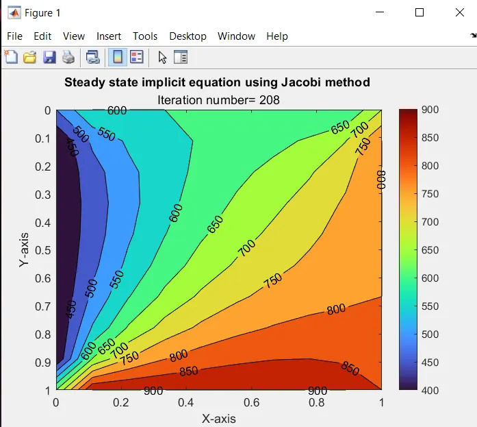
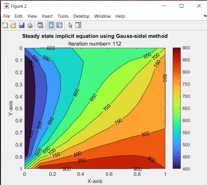
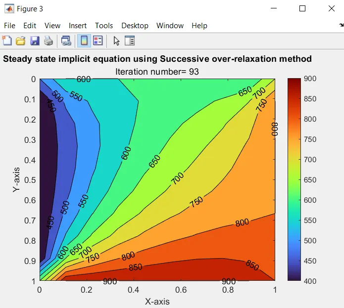
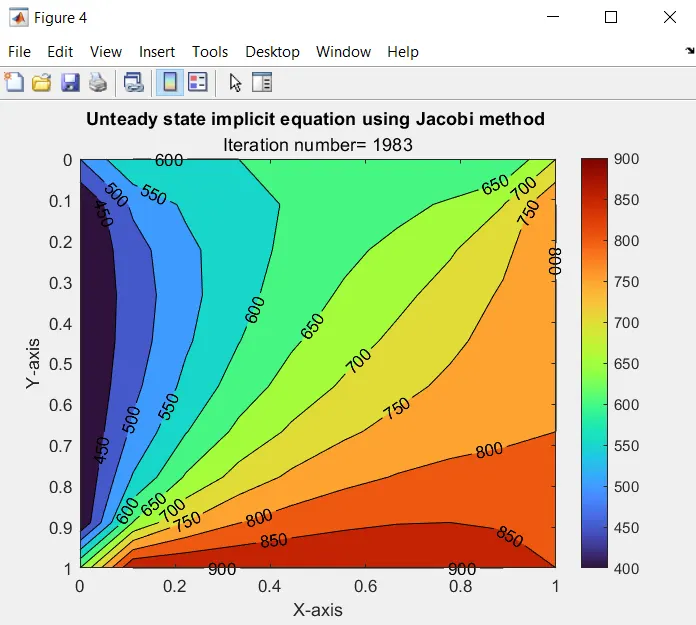
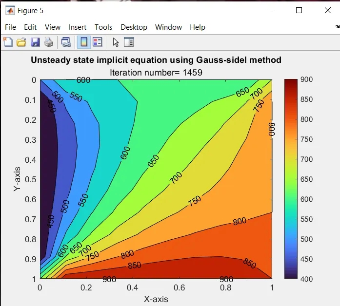
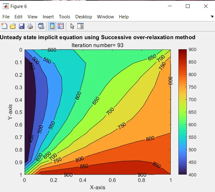
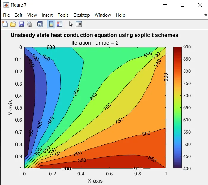
Sr. No.	Iteration method	Iteration number
1.	Steady-state implicit-Jacobi	208
2.	Steady-state implicit-Gauss-seidel	112
3.	Steady-state implicit-Successive over-relaxation	93
4.	Unsteady state implicit - Jacobi	1983
5.	Unsteady state implicit -Gauss-sidel	1459
6.	Unsteady state implicit -successive over-relaxation	93
7.	Unsteady state explicit	2

As seen from the above table, computational time as well as a number of iteration for Jacobi>GS>SOR for both steady and transient schemes.

Conclusion:

The Stability Issue

The principal reason for using implicit solution methods, which are more complex to program and require more computational effort in each solution step, is to allow for large time-step sizes. Let Q be a quantity whose value Qn+1 we want to compute at time t=(n+1)dt, in terms of its value at time t=ndt, i.e., Qn+1=Qn+dtS, where S is the rate of change in Q.

In an explicit numerical method, S would be evaluated in terms of known quantities at the previous time step n. An implicit method, in contrast, would evaluate some or all of the terms in S in terms of unknown quantities at the new time step n+1.

Numerical stability has to do with the behavior of the solution as the time-step dt is increased. If the solution remains well behaved for arbitrarily large values of the time step, the method is said to be unconditionally stable. This situation never occurs with explicit methods, which are always conditionally stable.

In an implicit formulation, a solution for the unknowns at new time step n+1 may be obtained for any size time step.

The Accuracy Issue

When dt is sufficiently small only one iteration is necessary for convergence, which leads to Qn+1=Qn+dt/(1+Cdt)Sn(C is a positive coefficient characterizing all the terms in the original equation). This shows that the implicit formulation adds a smaller change to Q in a one-time step than would occur in an explicit method because of the under-relaxation factor A=1/(1+Cdt) that multiplies the time step(A is relaxation coefficient).