Week 3.5 - Deriving 4th order approximation of a 2nd order derivative using Taylor Table method
Fourth order approximations of the second-order derivatives:
No. of nodes, N= P+Q
Where, P is the order of derivative
Q is the order of approximation
1. Central difference scheme:
No. of nodes, N = P+Q-1
= 2+4-1
= 5
Approximations for central difference scheme:
gradx^2frac(d^2u)(dx^2) = af(i-2)+bf(i-1)+cf(i)+df(i+1)+ef(i+2)
Using taylor series expansion:
|
gradx^2f’’(i) |
f(i) |
gradxf’(i) |
gradx^2f’’(i) |
gradx^3f’’’(i) |
gradx^4’’’’f(i) |
|
af(i-2) |
a |
-2a |
2a |
frac(-4a)3 |
frac(-2a)3 |
|
bf(i-1) |
b |
-b |
frac(b)2 |
frac(-b)6 |
frac(b)24 |
|
cf(i) |
c |
0 |
0 |
0 |
0 |
|
df(i+1) |
d |
d |
farc(d)2 |
frac(d)6 |
frac(d)24 |
|
ef(i-+2) |
e |
2e |
2e |
frac(4e)3 |
2e/3 |
|
sum |
0 |
0 |
1 |
0 |
0 |
we have matrix:
A.X=B
[[1,1,1,1,1],[-2,-1,0,1,2],[2,1/2,0,1/2,2],[4/3,1/6,0,1/6,4/3],[2/3,1/24,0,1/24,2/3]] . [[a],[b],[c],[d],[e]] =
[[0],[0],[1],[0],[0]]
By using matrix inversion method:
X = inv(A)*B
We get unknown values : a=-0.0833, b=1.3333, c=-2.5000, d=1.3333 e=-0.0833
2. Skewed right-sided difference scheme
In right side skew scheme:
No. of nodes, N= P+Q
= 2+4
= 6
Approximations for skewed right-sided difference scheme:
gradx^2frac(d^2u)(dx^2) = af(i)+bf(i+1)+cf(i+2)+df(i+3)+ef(i+4)+gf(i+5)
Using taylor series expansion
|
gradx^2f’’(i) |
f(i) |
gradxf’(i) |
gradx^2f’’(i) |
gradx^3f’’’(i) |
gradx^4’’’’f(i) |
gradx^5f’’’’’(i) |
|
af(i) |
a |
0 |
0 |
0 |
0 |
0 |
|
bf(i+1) |
b |
b |
b/2 |
b/6 |
b/24 |
b/120 |
|
cf(i+2) |
c |
2c |
frac(4c)2 |
frac(8c)6 |
frac(16c)24 |
frac(32c)120 |
|
df(i+3) |
d |
3d |
frac(9d)2 |
frac(27d)6 |
frac(81d)24 |
frac(243d)120 |
|
ef(i+4) |
e |
4e |
frac(16e)2 |
frac(64e)6 |
frac(256e)24 |
frac(1024e)120 |
|
gf(i+5) |
g |
5g |
frac(25g)2 |
frac(125g)6 |
frac(625g)24 |
frac(3125g)120 |
|
sum |
0 |
0 |
1 |
0 |
0 |
0 |
we have matrix:
A.X=B
[[1,2,3,4,5],[1/2,2,9/2,8,25/2],[1/6,4/3,27/6,32/3,125/6],[1/24,2/3,27/8,32/3,625/24],[1/120,4/15,243/120,1024/120,3125/120]] . [[a],[b],[c],[d],[e]] =
[[0],[0],[1],[0],[0]]
By using matrix inversion method:
X = inv(A)*B
We get unknown values: a = 3.7500, b=-12.8333, c=17.8333, d=-13.0000 e=5.0833 g=-0.8333
3. Skewed left-sided difference scheme
In left-side skew scheme:
No. of nodes, N= P+Q
= 2+4
= 6
Approximations for skewed left-sided difference scheme:
gradx^2frac(d^2u)(dx^2) = af(i-5)+bf(i-4)+cf(i-3)+df(i-2)+ef(i-1)+gf(i)
Using taylor series expansion:
|
gradx^2f’’(i) |
f(i) |
gradxf’(i) |
gradx^2f’’(i) |
gradx^3f’’’(i) |
gradx^4’’’’f(i) |
gradx^5f’’’’’(i) |
|
af(i-5) |
a |
-5a |
frac(25a)2 |
frac(-125a)6 |
frac(625a)24 |
frac(-3125a)120 |
|
bf(i-4) |
b |
-4b |
frac(16b)2 |
frac(-64b)6 |
frac(256b)24 |
frac(-1024b)120 |
|
cf(i-3) |
c |
-3c |
frac(9c)2 |
frac(-27c)6 |
frac(81c)24 |
frac(-243c)120 |
|
df(i-2) |
d |
-2d |
farc(4d)2 |
frac(-8d)6 |
frac(16d)24 |
frac(-32d)120 |
|
ef(i-1) |
e |
-e |
e/2 |
-e/6 |
e/24 |
-e/120 |
|
gf(i) |
g |
0 |
0 |
0 |
0 |
0 |
|
sum |
0 |
0 |
1 |
0 |
0 |
0 |
we have matrix:
A.X=B
[[-5,-4,-3,-2,-1],[25/2,8,9/2,2,1/2],[-125/6,32/3,9/2,4/3,-1/6],[625/24,32/3,27/8,2/3,1/24],[-625/24,256/30,-27/14,-4/15,1/20]] . [[a],[b],[c],[d],[e]] =
[[0],[0],[1],[0],[0]]
By using matrix inversion method:
X = inv(A)*B
We get unknown values: a=-0.8333, b=5.0833, c=-13.0000, d=17.8333 e=-12.8333 g=3.7500
Result:
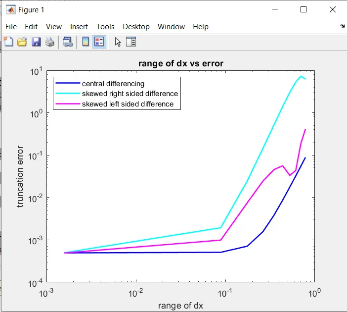
Conclusion:
Central difference < Right Skewed ≅ Left Skewed
Why a skewed scheme is useful?
Ans: In systems having numerical stencil with non symmetric points skewed scheme can be useful.
What can a skewed scheme do that a CD scheme cannot?
Ans: CDS is applicabe only at the center of mesh and cannot not be used at the boundary nodes because right and left nodes are not available.Sskewed differencing scheme can be used to find right and left sided boundary nodes.
Main code:
clear all
close all
clc
%value of x
x= pi/3;
%range of dx
dx= linspace(pi/4,pi/2000,10);
%for loop
for i=1:length(dx)
central_differencing(i) = fourth_order_central_differencing(x,dx(i));
right_sided_skew(i) = fourth_order_right_sided_skew(x,dx(i));
left_sided_skew(i) = fourth_order_left_sided_skew(x,dx(i));
end
%plotting
figure(1)
loglog(dx,central_differencing,'LineWidth',1.5,'color','central_differencing(i)')
hold on
loglog(dx,right_sided_skew,'LineWidth',1.5,'color','c')
hold on
loglog(dx,left_sided_skew,'LineWidth',1.5,'color','m')
xlabel('range of dx')
ylabel('truncation error')
title('range of dx vs error')
legend('central differencing','skewed right sided difference','skewed left sided difference','location','northwest')
Function code for central differencing:
function Error_central_differencing = fourth_order_central_differencing(x,dx)
% analytic function = exp(x)*cos(x)
% analytic derivative
%f''(x) = -2*exp(x)*sin(x)
analytical_derivative = -2*exp(x).*sin(x);
%numerical derivative
%central differencing
central_differencing=(((-0.0833)*((exp(x-(2*dx))).*(cos(x-(2*dx)))))+((1.3333)*((exp(x-dx)).*(cos(x-dx))))-((2.5000)*((exp(x)).*(cos(x))))+((1.3333)*((exp(x+dx)).*(cos(x+dx))))-((0.0833)*((exp(x+(2*dx))).*(cos(x+(2*dx))))))/(dx.^2);
%error
Error_central_differencing = abs(central_differencing- analytical_derivative);
end
Function code for right-sided differencing:
function Error_right_sided_skew = fourth_order_right_sided_skew(x,dx)
% analytic function = exp(x)*cos(x)
% analytic derivative
%f''(x) = -2*exp(x)*sin(x)
analytical_derivative = -2*exp(x).*sin(x);
%numerical derivative
%central differencing
right_sided_skew = ((3.7500*exp(x).*cos(x))-(12.8333*exp(x+dx).*cos(x+dx))+(17.8333*exp(x+(2*dx)).*cos(x+(2*dx)))-(13.0000*exp(x+(3*dx)).*cos(x+(3*dx))) +(5.0833*exp(x+(4*dx)).*cos(x+(4*dx)))-(0.8333*exp(x+(5*dx)).*cos(x+(5*dx)))) /(dx.^2);
%error
Error_right_sided_skew = abs(right_sided_skew- analytical_derivative);
end
Function code for left-sided differencing:
function Error_left_sided_skew = fourth_order_left_sided_skew(x,dx)
% analytic function = exp(x)*cos(x)
% analytic derivative
%f''(x) = -2*exp(x)*sin(x)
analytical_derivative = -2*exp(x).*sin(x);
%numerical derivative
%central differencing
left_sided_skew = (((-0.8333)*((exp(x-(5*dx))).*(cos(x-(5*dx)))))+((5.0833)*((exp(x-(4*dx))).*(cos(x-(4*dx)))))-((13.0000)*((exp(x-(3*dx))).*(cos(x-(3*dx)))))+((17.8333)*((exp(x-(2*dx))).*(cos(x-(2*dx)))))-((12.8333)*((exp(x-dx)).*(cos(x-dx))))+((3.7500)*((exp(x)).*(cos(x)))))/(dx.^2);
%error
Error_left_sided_skew = abs(left_sided_skew- analytical_derivative);
end