Week 9 - FVM Literature Review

Objective: The objective is to define what is Finite Volume Method(FVM), differentiate between FDM & FVM, & describe the need for interpolation schemes and flux limiters in FVM.

Finite Volumre Method (FVM):

The finite volume method solves partial differential equations that calculate the values of the conserved variables averaged across the volume. One advantage of the finite volume method over finite difference methods is that it does not require a structured mesh (although a structured mesh can also be used). Furthermore, the finite volume method is preferable to other methods as a result of the fact that boundary conditions can be applied non-invasively. This is true because the values of the conserved variables are located within the volume element, and not at nodes or surfaces. Finite volume methods are especially powerful on coarse nonuniform grids and in calculations where the mesh moves to track interfaces or shocks.

FDM LImitatioions

• FDM is very simple and effective over structured grids. It is especially easy to obtain higher-order schemes on regular grids. 
• The disadvantage of the FDM is that certain conservation laws are not enforced unless special care is taken.
• The restriction to simple geometries is a significant disadvantage if complex flows are specified in FDM.
• Furthermore, the FDM uses a topologically square network of lines to construct the discretization of the PDE.
• Tough to implement in complex geometry where it needs complex mapping and mapping makes governing equations even tougher
• The finite-difference method is more difficult to use for handling material discontinuities.
• It does not lend itself to local grid refinement or anything similar to “adaptive mesh refinement.” This may be needed to resolve local rapid variations in solutions such as around a corner of a complex shape.

Advantages of FVM over FDM

• FVM can accommodate any type of grid, so it is suitable for complex geometries.
• FVM is similar to FDM but the method (FVM) integrates the differential equation over a control volume and discretizes the domain. Conservation of mass, momentum, energy is ensured at each cell/finite volume level. Since we have integrated the differential equation discretization is mathematically a valid one
• Using Governing Equation in Conservative form with FV approach to solve any problem ensures conservation of all the properties in each cell/control volume.
• In FVM, fluxes are integrated and the resultant is set to zero, so flux is conserved. FVM handles almost any PDEs and complex domain.
• FVM accuracy is based on the order of the polynomial used. FVM can also produce any order accurate numerical solution similar to FDM.

Interpolation schemes in FVM

The approximation of surface and volume integrals requires variables at locations other than the computational nodes of the CV. Values at these locations are obtained using interpolation schemes.

Various interpolation schemes are 

• Upwind Interpolation Schemes
• Linear Interpolation Schemes
• QUICK - Quadratic Upwind Interpolation Schemes
• Hybrid Interpolation
• Total Variation Diminish

Upwind Interpolation Schemes 

It is used in the numerical method in CFD for the convection-diffusion problems. This scheme is specifically for Peclet numbers greater than 2 and less than -2.

The upwind interpolation scheme approximation the value of a variable at the east face of the control volume.

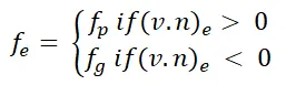
The interpolation scheme is equivalent to using backward or forward finite difference approximation. It is the first order accurate and is numerically diffusive with a coefficient of numerical diffusion

By taking into account the direction of flow, the upwind differencing scheme overcomes that inability of the central difference scheme. This scheme is developed for strong convection flows with suppressed diffusion effects.

Linear interpolation

The linear interpolation is equivalent to the use of the central difference formula of the first-order derivative and hence it is second-order accurate whose accuracy is very good but we might have one small problem for advection dominates situations, that this scheme may produce oscillatory solutions. This scheme leads to a simple approximation for evaluation of gradients required for evaluation of diffusion flux

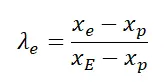
Function which would depend on relative locations of the computational nodes E and P with respect to the eastern face.

Quadratic upwind interpolation

The quadratic upwind interpolation is three order scheme, it is derived from the polynomial fitting. It is also represented as QUICK interpolation on a uniform Cartesian is given by

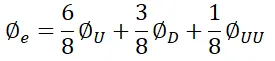
Where D, C, and UU donate the downstream, the first upstream and second upstream node respectively. OUICK scheme is prone to oscillation because of the third-order scheme

Hybrid Interpolation

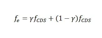
This scheme is a combination of upwind interpolation scheme and central distribution scheme based on the local peclet number

Total Variation Diminish

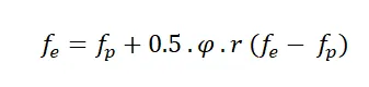
Ψ = Local flux limiter

r = Specified function which depends upon the local flow conditions

Flux limiters in FVM

Flux limiter is introduced in the higher-order differencing scheme to prevent unwanted oscillations and ensure bounded results, It is used to maintain the property of the scheme. It avoids the spurious oscillations that would occur with high order spatial discretization scheme due to shocks, discontinuities, or sharp changes in the solution domain. The use of flux limiters, together with an appropriate high-resolution scheme, makes the solutions total variation diminishing (TVD).

Fluz limiters usually restrict the results to some realistic values.

Consider 1D Semi-discrete scheme,

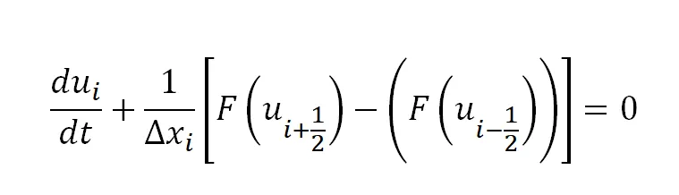
where  and 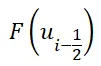 represent edge flux for the ith cell. If these edge fluxes can be represented by low and high-resolution schemes, then a flux limiter can be switched between these schemes depending upon the gradient close to the particular cell, as follows,

where,

=  low-resolution flux

= high-resolution flux

= flux limiter function

 and r represents the ratio of successive gradients on the solution mesh.

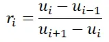
The limiter function is constrained to be greater than or equal to zero.

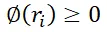
Therefore, when the limiter is equal to zero, the flux is represented by a low-resolution scheme. Similarly, when the limiter is equal to 1, it is represented by a high-resolution scheme.