Week 7 - Simulation of a 1D Super-sonic nozzle flow simulation using Macormack Method
Objective: To simulate the isentropic flow through a quasi 1D subsonic-supersonic nozzle by deriving using both the conservation and non-conservation forms of the governing equations and solve them using the MacCormack's technique.
Problem Description:
A steady-state isentropic flow through the convergent-divergent nozzle is considered. The inlet to the nozzle is considered from a reservoir. It is considered that near to the inlet, the velocity is very small almost equivalent to zero but not equal to zero and the cross-section area is almost infinity. The flow expands isentropic to supersonic speeds at the nozzle exit. The flow is locally subsonic in the convergent section of the nozzle, sonic at the throat & Supersonic at the divergent section of the nozzle.
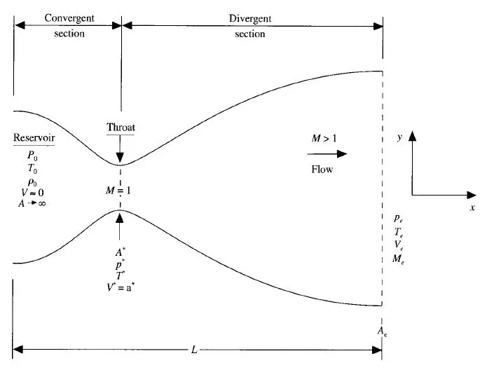
It is assumed that, at a given section, the cross-section area is uniform across that section. Hence, although the area of the nozzle changes as a function of distance along with nozzle, and therefore in reality the flow field is two-dimensional, we assume that the flow property varies only with respect to x. This tantamount to assuming uniform flow properties across any given cross-section. Such flow is defined as the quasi-one-dimensional flow.
The governing continuity, momentum & energy equations for this quasi-one-dimensional, steady isentropic flow can be expressed as
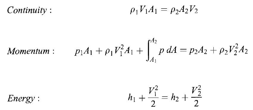
where subscripts 1 & 2denotes different locations along with the nozzle.
Non-Conservative Method:
Referring to the book on CFD by John Anderson, Equations for calculating primitive variables & for Initial and boundary conditions are derived.
Matlab Code is written following the steps of MacCormack's technique and is executed for its correctness with respect to the solution in the book.
Matlab Code - Non-Conservative Method
% non conservative Method
clear all
close all
clc

% inputs
n = 31;
x = linspace (0,3,n);
dx = x(2) - x(1);
gamma = 1.4;
C = 0.5;

% Calculate initial Profiles
rho = 1 - 0.3146*x;
t = 1 - 0.2314*x; % temperature
v = (0.1 + 1.09*x).*t.^0.5;

% area
a = 1+2.2* (x-1.5).^2;

% time step
nt = 1400;
dt = 0.02;
time = 0;

ct =1;

% Outer Time Loop
for k = 1:nt

    dt = min(C.*(dx./(sqrt(t)+v)));

% Copying old values
    rho_old = rho;
    v_old = v;
    t_old = t;

    % predictor Method
    for j = 2:n-1
        dvdx = (v(j+1) - v(j))/dx;
        drhodx = (rho(j+1)-rho(j))/dx;
        dtdx = (t(j+1)-t(j))/dx;
        dlogadx = (log(a(j+1)) - log(a(j)))/dx;

        % Continuity Equation
        drhodt_p(j) = -rho(j)*dvdx-rho(j)*v(j)*dlogadx-v(j)*drhodx;

        % Momentum Equation
        dvdt_p(j) = -v(j)*dvdx-(1/gamma)*(dtdx + (t(j)/rho(j))*drhodx);

        % Energy Equation
        dtdt_p(j) = -v(j)*dtdx-(gamma-1)*t(j)*(dvdx + v(j)*dlogadx);

        % Solution Update

        rho(j) = rho(j) + drhodt_p(j)*dt;
        v(j) = v(j) + dvdt_p(j)*dt;
        t(j) = t(j) + dtdt_p(j)*dt;

    end

    % Corrector Method
    for j = 2:n-1

        dvdx = (v(j) - v(j-1))/dx;
        drhodx = (rho(j)-rho(j-1))/dx;
        dtdx = (t(j)-t(j-1))/dx;
        dlogadx = (log(a(j)) - log(a(j-1)))/dx;

        % Continuity Equation
        drhodt_c(j) = -rho(j)*dvdx-rho(j)*v(j)*dlogadx-v(j)*drhodx;

        % Momentum Equation
        dvdt_c(j) = -v(j)*dvdx-(1/gamma)*(dtdx + (t(j)/rho(j))*drhodx);

        % Energy Equation
        dtdt_c(j) = -v(j)*dtdx-(gamma-1)*t(j)*(dvdx + v(j)*dlogadx);

    end

    % Compute Average time Derivative

    drhodt = 0.5 * (drhodt_p + drhodt_c);
    dvdt = 0.5 * (dvdt_p + dvdt_c);
    dtdt = 0.5 * (dtdt_p + dtdt_c);

    %Final Solution Update
    for  i=2:n-1
        rho(i) = rho_old(i) + drhodt(i)*dt;
        v(i) = v_old(i) + dvdt(i)*dt;
        t(i) = t_old(i) + dtdt(i)*dt;

    end

    % Applying Boundary Conditions
    % Inlet
    v(1) = 2*v(2) - v(3);

    % outlet
    rho(n) = 2*rho(n-1) -rho(n-2);
    v(n) = 2*v(n-1) -v(n-2);
    t(n) = 2*t(n-1) -t(n-2);

    m_f_r = rho .* v.* a;
    Mach_Number = v./(t.^0.5);
    p = rho.*t;

    figure(1)
    subplot(6,1,1)
    plot (x,Mach_Number)
    title(sprintf('Mach Number at Timestep %d & time =%d sec',k,time))

    subplot(6,1,2)
    plot(x,v)
    title(sprintf('Velocity at Timestep %d & time =%d sec',k,time))

    subplot(6,1,3)
    plot (x,p)
    title(sprintf('Pressure at Timestep %d & time =%d sec',k,time))

    subplot(6,1,4)
    plot (x,rho)
    title(sprintf('Density at Timestep %d @ time =%d sec',k,time))

    subplot(6,1,5)
    plot (x,t)
    title(sprintf('Temperature at Timestep %d & time =%d sec',k,time))

    subplot(6,1,6)
    plot (x,m_f_r)
    title(sprintf('Mass Flow Rate at Timestep %d & time =%d sec',k,time))
    pause(0.00003)

    M(ct)=getframe(gcf);
    ct = ct+1;
    % time step updating
    time = time + dt;

end

% Writing movie file
movie(M)
videofile=VideoWriter('Non_Conservative_Method.avi','uncompressed AVI');
open(videofile)
writeVideo(videofile,M)
close(videofile)
Code Explanations
The code starts with the default command for clearing all, closing all & clearing the command window. Then the basic input values of the problems are provided.
As the first step, The primitive variables are initialized following which the area & time steps are provided. ct value is introduced with is used to capture frames for recording the video.
The main "for" loop with Time as the operating function is started. as the time step value varies with respect to the primitive variable, This time step size is calculated.
Predictor Method equations are solved now and to solve this suitable for loop is used and also separate equations for splitting up of the main equation to avoid flaws. Continuity Equation, Momentum Equation & Energy Equation are solved in this step & the primitive variables are updated with respect to the primitive equations.
Following this, the Corrector method is done as the next step. Like the predictor method, to solve this corrector method, suitable for loop is used and also separate equations for splitting up of the main equation to avoid flaws. The continuity Equation, Momentum Equation & Energy Equation are solved in this step.
The average time derivative is calculated following which the final solution is also updated. by using suitable for loops.
Boundary conditions need to be updated now. In the inlet, the velocity is updated and at the outlet, all the primitive variables are updated by using the values at adjacent nodes.
Plotting of all the variables is done and the frames are saved which will be used to prepare the animation of the solution and the time step value is updated to the next value.
The time loop is ended here.
The movie file is written by using the frames captured while solving the equations inside the time loop.
The results of the Non- Conservative method are discussed later part of the report.
Conservative Method:
Referring to the book on CFD by John Anderson, Equations for calculating primitive variables & for Initial and boundary conditions are derived.
Matlab Code is written following the steps of MacCormack's technique and is executed for its correctness with respect to the solution in the book.
Matlab Code - Conservative Method:
% Conservative Method
clear all
close all
clc

% inputs
n = 31;
x = linspace (0,3,n);
dx = x(2) - x(1);
gamma = 1.4;
C = 0.5;

% area
a = 1+2.2* (x-1.5).^2;

% Calculate initial Profiles

for i=1:n

    if 0 <= x(i) && x(i) <= 0.5
        rho(i) = 1;
        t(i) = 1;

    elseif 0.5 <= x(i) && x(i) <= 1.5
        rho(i) = 1 - (0.366*(x(i) - 0.5));
        t(i) = 1 - (0.167*(x(i) - 0.5));

    elseif 1.5 <= x(i) && x(i) <= 3.5
        rho(i) = 0.634 - (0.3879*(x(i) - 1.5));
        t(i) = 0.833 - (0.3507*(x(i) - 1.5));
    end
end

v = 0.59./(rho.*a);

% Corresponding Initial Conditions
U1 = rho.*a;
U2 = rho.*a.*v;
U3 = rho.*((t./(gamma-1))+ (gamma.*(v.^2)./2)).*a;

% Time Step
dt = min(C.*(dx./(sqrt(t)+v)));
nt = 1400;
time = 0;

% Initialising the variables
U1_p=U1;
U2_p=U2;
U3_p=U3;
U1_c=U1;
U2_c=U2;
U3_c=U3;
rho_p = rho;
t_p = t;

ct = 1;

 for k=1:nt
    dt = min(C.*(dx./(sqrt(t)+v)));

    % FLux Terms
    F1 = U2;
    F2 = ((U2.^2)./U1)+((gamma-1)/gamma)*(U3-(gamma/2*(U2.^2)./(U1)));
    F3 = (gamma* U2.*U3./U1)-(gamma/2*(gamma-1)*(U2.^3)./((U1.^2)));

    for i = 2:n-1
        % Source Term
        J2(i) = (1/gamma)*rho(i)*t(i)*((a(i+1)-a(i))/dx);

        % predictor Method
        dU1dt_p(i) = -(F1(i+1) - F1(i))/dx;
        dU2dt_p(i) = -((F2(i+1) - F2(i))/dx)+J2(i);
        dU3dt_p(i) = -(F3(i+1) - F3(i))/dx;

        % Predicted U values
        U1_p(i) = U1(i) + (dU1dt_p(i) *dt);
        U2_p(i) = U2(i) + (dU2dt_p(i) *dt);
        U3_p(i) = U3(i) + (dU3dt_p(i) *dt);
    end

    % Predicted Primitive Values
    for i = 2:n-1
        rho_p(i) = U1_p(i)/a(i);
        t_p(i) = (gamma-1)*((U3_p(i)/ U1_p(i))-((gamma/2)*((U2_p(i)/ U1_p(i))^2)));
    end

    % FLux Terms
    F1 = U2_p;
    F2 = ((U2_p.^2)./U1_p)+((gamma-1)/gamma)*(U3_p-(gamma/2*(U2_p.^2)./(U1_p)));
    F3 = (gamma* U2_p.*U3_p./U1_p)-(gamma/2*(gamma-1)*(U2_p.^3)./((U1_p.^2)));

    for i = 2:n-1

        % Source Term - Corrected
        J2(i) = (1/gamma)*rho_p(i)*t_p(i)*((a(i)-a(i-1))/dx);

        % Corrected U Values
        dU1dt_c(i) = -(F1(i) - F1(i-1))/dx;
        dU2dt_c(i) = -((F2(i) - F2(i-1))/dx)+J2(i);
        dU3dt_c(i) = -(F3(i) - F3(i-1))/dx;
    end

    % Average Time Derivative
    dU1dt_av = (dU1dt_p + dU1dt_c)/2;
    dU2dt_av = (dU2dt_p + dU2dt_c)/2;
    dU3dt_av = (dU3dt_p + dU3dt_c)/2;

    % Corrected Primitive Values

    for i= 2:n-1
        U1_c(i) = U1(i) + (dU1dt_av(i)*dt);
        U2_c(i) = U2(i) + (dU2dt_av(i)*dt);
        U3_c(i) = U3(i) + (dU3dt_av(i)*dt);
    end

      % Applying Boundary Conditions
        % Inlet
        U2_c(1) = 2*U2_c(2) - U2_c(3);
        v(1) =  U2_c(1)/U1_c(1);
        U3_c(1) = rho(1)*((t(1)/(gamma-1))+ (gamma*(v(1)^2)/2))*a(1);

        % outlet
        U1_c(n) = 2*U1_c(n-1) -U1_c(n-2);
        U2_c(n) = 2*U2_c(n-1) -U2_c(n-2);
        U3_c(n) = 2*U3_c(n-1) -U3_c(n-2);

    for i = 1:n
        % Corrected Primitive Values
        rho(i) =  U1_c(i)/a(i);
        v(i) =  U2_c(i)/U1_c(i);
        t(i) = (gamma-1)* ((U3_c(i)/U1_c(i)) - (gamma*(v(i)^2)/2));
    end

        m_f_r = rho .* v.* a;
        Mach_Number = real(v./(t.^0.5));
        p = rho.*t;

        % Copy of U terms

        U1 = U1_c;
        U2 = U2_c;
        U3 = U3_c;

        U1_p = U1;
        U2_p = U2;
        U3_p = U3;

       % k = 1
        figure(1)
        subplot(6,1,1)
        plot (x,Mach_Number)
        title(sprintf('Mach Number at Timestep %d & time =%d sec',k,time))

        subplot(6,1,2)
        plot(x,v)
        title(sprintf('Velocity at Timestep %d & time =%d sec',k,time))

        subplot(6,1,3)
        plot (x,p)
        title(sprintf('Pressure at Timestep %d & time =%d sec',k,time))

        subplot(6,1,4)
        plot (x,rho)
        title(sprintf('Density at Timestep %d @ time =%d sec',k,time))

        subplot(6,1,5)
        plot (x,t)
        title(sprintf('Temperature at Timestep %d & time =%d sec',k,time))

        subplot(6,1,6)
        plot (x,m_f_r)
        title(sprintf('Mass Flow Rate at Timestep %d & time =%d sec',k,time))

        pause(0.001)

        M(ct)=getframe(gcf);
        ct = ct+1;
        % time step updating
        time = time + dt

 end
 % Writing movie file
movie(M)
videofile=VideoWriter('Conservative_Method.avi','uncompressed AVI');
open(videofile)
writeVideo(videofile,M)
close(videofile)
Code Explanations
As like the code for the Non-Conservative method, The code starts with the default command for clearing all, closing all & clearing the command window. Then the basic input values of the problems are provided along with the cross-section area.
As the first step, The primitive variables are initialized. These initial values depend on the value of "x" at that point and so suitable for loops, if & if-else conditions is used to initialize them.
With the initial primitive variables, Initial values of U1, U2 & U3 are calculated.
Time steps information is provided. Other variables that are to be used inside the calculation is initialized to reduce the solving time. "ct" value is introduced with is used to capture frames for recording the video.
The main "for" loop with Time as the operating function is started. as the time step value varies with respect to the primitive variable, This time step size is calculated as the first step inside the execution of for loop.
Flux terms are calculated using the values of U1, U2 & U3 and using these values, Predictor values are calculated. Predicted primitive variables are calculated which are to be used in the further steps
Flux terms are again updated to use them for the calculation of the corrected values
The average time derivative is calculated following which the final solution is also updated. by using suitable for loops.
Boundary conditions need to be updated now. In the inlet, the velocity is updated and at the outlet, all the primitive variables are updated by using the values at adjacent nodes.
U1, U2 & U3 are recalculated with respect to the updated primitive variables.
Plotting of all the variables is done and the frames are saved which will be used to prepare the animation of the solution and the time step value is updated to the next value.
The time loop is ended here.
The movie file is written by using the frames captured while solving the equations inside the time loop.
The results of the Conservative method are discussed later part of the report.
Results
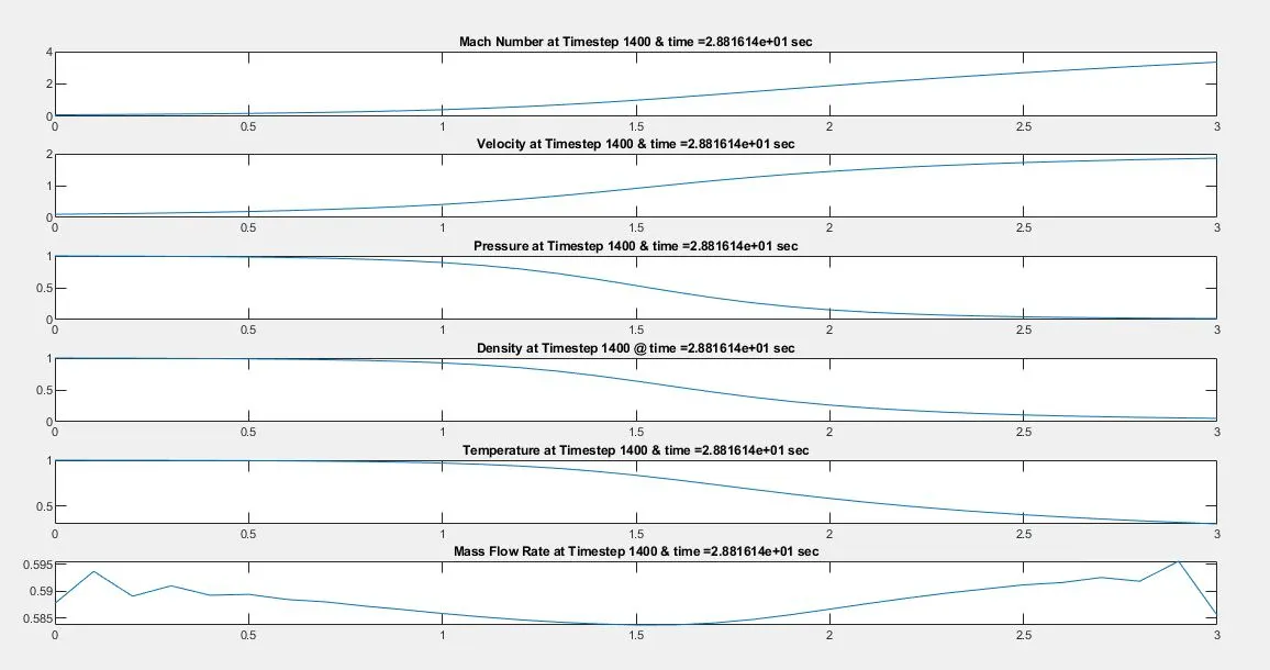
Non- Conservative Method
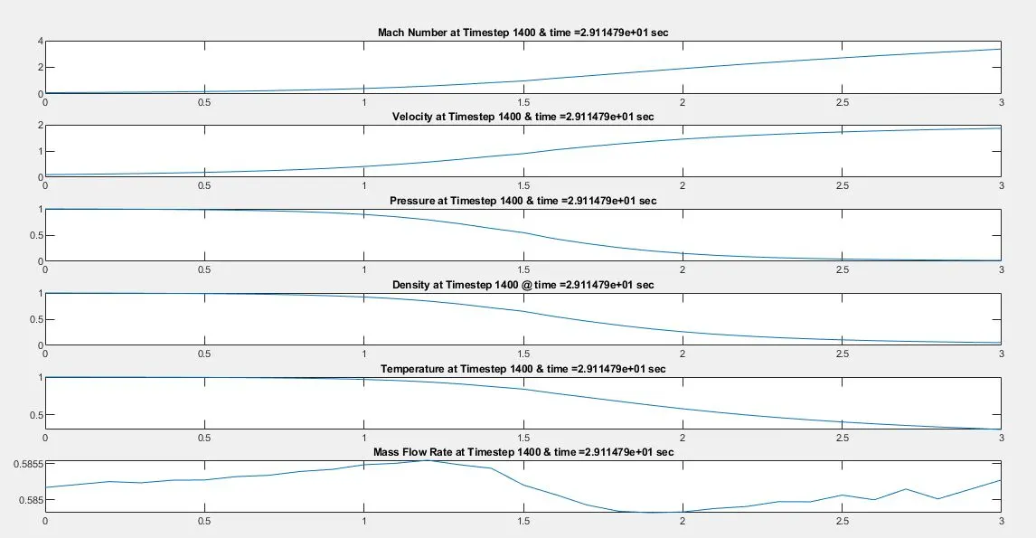
Conservative Method
Value of Primitive variables along time:
Non-Conservative Method (n= 31)
From the above plots we can notice that all the primitive variables are almost converged. End time of analysis varies because of the calculation of dt inside the "for" loop.
The solution which was given as per the book on CFD by John Anderson:
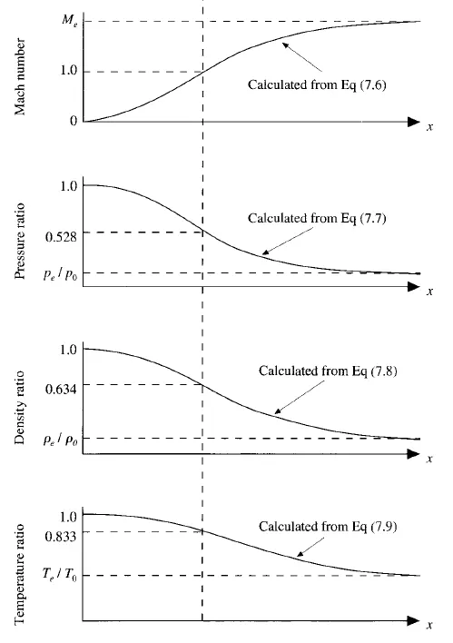
On comparison of the solution obtaiined, with the solution in the book, we can conclude that this code work perfect.
Grid Independence Test
As we have the exact solution, we can the calculated results with the standard one. In other scenarios, where we dont have exact solution, indrder to confirm the correctness of solution, we need to perform this grid independence test.
Here, instead of 31 nodes, 62 nodes are used to calculate the results. Same code is executed with n= 62 and the results are plotted below:
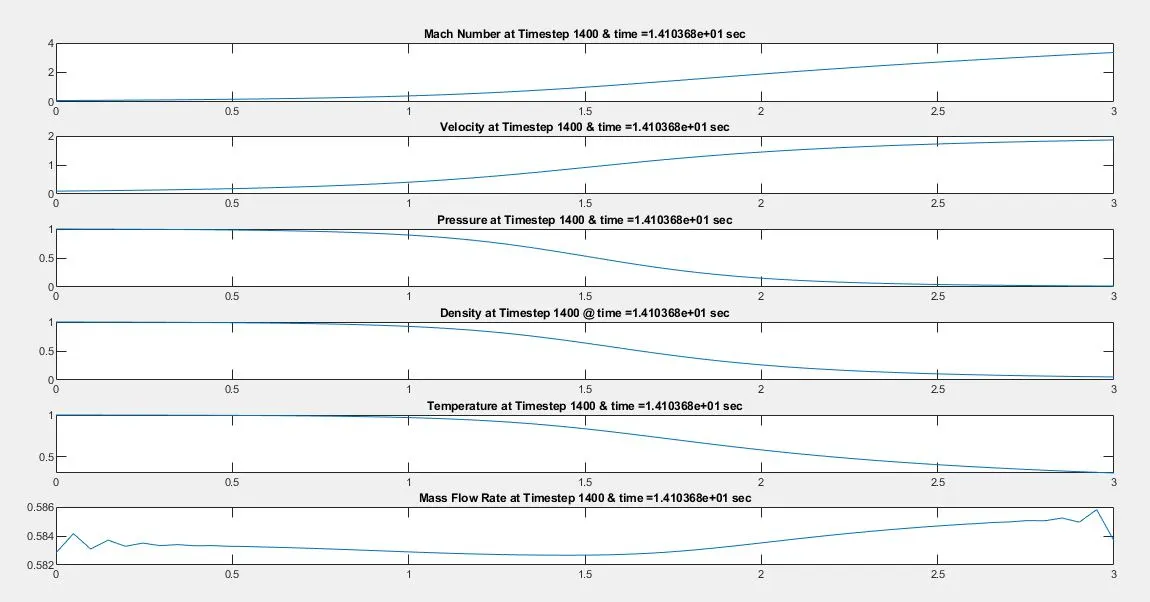
Non- Conservative Method
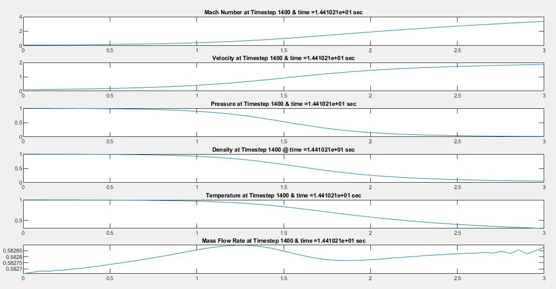
Conservative Method
Value of Primitive variables along time:
Non-Conservative Method ( n = 62)
On comparing the results with n = 31 & n = 62, the results are almost the same and there is no significant difference is seen in the plot. From this we can say that the results are grid independent i.e ., the results are not dependent on the grid.