Week 9 - FVM Literature Review

What is the Finite Volume Method? (FVM)

• The finite volume method is a discretization method that is well suited for the numerical simulation of
  various types (elliptic, parabolic, or hyperbolic) of conservation laws; it has been extensively
  used in several engineering fields, such as fluid mechanics, heat and mass transfer, or petroleum engineering.
• The finite volume method is locally conservative because it is based on a “ balanced” approach: a local balance
  is written on each discretization cell which is often called “control volume”
• An additional feature is the local conservative of the numerical fluxes, that is the numerical flux is conserved from one discretization cell to its neighbor. This last feature makes the finite volume method quite attractive when modeling problems for which the flux is of
  importance, such as in fluid mechanics, semi-conductor device simulation, heat, and mass transfer.

Finite Difference Method(FDM)

Finite Volume Method(FVM)

A finite difference method (FDM) discretization is based upon the differential form of the PDE to be solved. Each derivative is replaced with an approximate difference formula (that can generally be derived from a Taylor series expansion). The computational domain is usually divided into hexahedral cells (the grid), and the solution will be obtained at each nodal point. The FDM is easiest to understand when the physical grid is Cartesian, but through the use of curvilinear transforms the method can be extended to domains that are not easily represented by brick-shaped elements The resulting approximate solution is discrete, but the variables are typically placed at cell centers rather than at nodal points.

A finite volume method (FVM) discretization is based upon an integral form of the PDE to be solved (e.g. conservation of mass, momentum, or energy). The PDE is written in a form that can be solved for a given finite volume (or cell). The computational domain is discretized into finite volumes and then for every volume, the governing equations are solved. The resulting system of equations usually involves fluxes of the conserved variable, and thus the calculation of fluxes is very important in FVM. FVM is generally expected to provide better conservation properties It does not require the use of structured grids, and the effort to convert the given mesh into a structured numerical grid internally is completely avoided

To describe the need for interpolation schemes and flux limiters in FVM

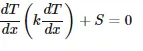
The approximation of volume and surface integrals may require values of the variable at locations other than the computational nodes at control volume. The 1D heat equation is:

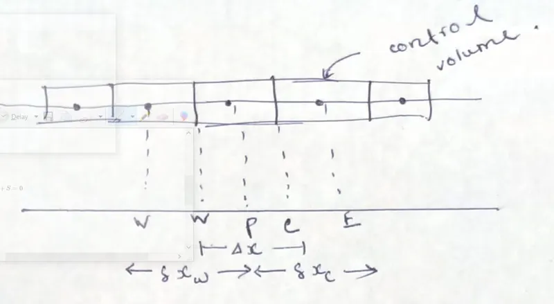
Step 1: Divide the domain into a finite-sized subdomain and each subdomain is represented by a grid point.

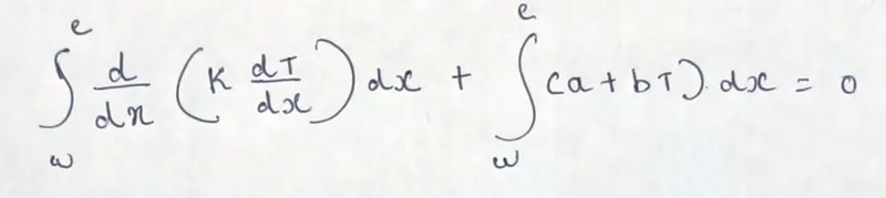
step 2: Integrate governing equation

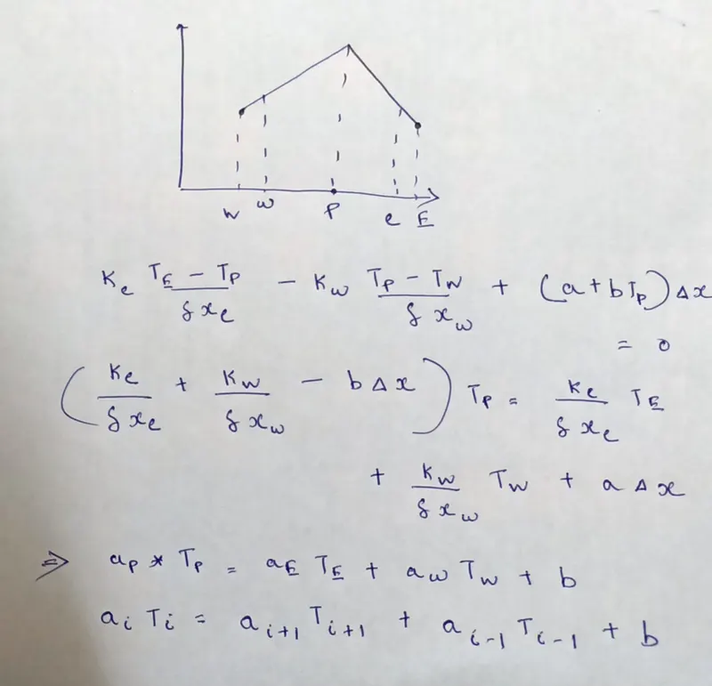
step 3: Consider a profile assumption for the dependent variable for evaluating the above integrals to express the results in terms of algebraic quantity at the grid points.a linear interpolation scheme is used to determine the temperature distribution along with the faces of grid points

The flux Limiter method tries to limit the contribution from the second-order correction near the discontinuity.